Simulation of Flow through a pipe in OpenFoam
Simulation of Flow through a pipe
Hagen-Poiseuille equation
In non fluid dynamics, the Hagen-Poiseuille equation is a physical law that gives the pressure drop in an incopressible and Newtonian fluid in laminar flow flowing through a long cylindrical pipe of constant cross section.
The assumption of the equation are
- The fluid is incompressible and Newtonian, which means, the viscosity property of fluid follows Newton’s law of viscosity, that is, τ=μdudy">τ=μdudyτ=μdudy
- There is no relative motion between fluid particles and solid boundaries, that is no slip of fluid at the solid boundary.
- The flow is laminar through a pipe of constant circular cross section that is substantially longer than its diameter
- There is no acceleration of fluid in the pipe.
Poiseuille’s Equation describes the pressure drop due to the viscosity of the fluid.
`ΔP=(8μLQ)/(πR^4)`ΔP=8μLQπR4=8πμLQA2">
Where
ΔP">ΔP is the pressure difference between the two ends
L is the length of pipe
μ">μ is the dynamic viscosity
Q is the volumetric flow rate
R is the pipe radius
A is the cross section of pipe
There are some limitation for Hagen-Poiseuille’s equations
- The equation dose not hold close to the pipe entrance.
- The equation fails in the limit of low viscosity, wide and/or short pipe. Low viscosity or a wide pipe may result in turbulent flow, making it necessary to use more complex models, such as the Darcy-Weisbach equation.
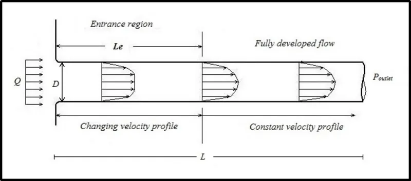
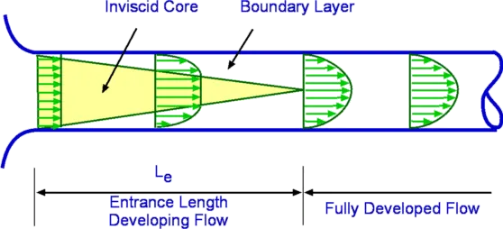
As fluid moves downstream from the entrance to a channel, its speed distribution or velocity profile changes in shape until it becomes fully developed. The length of an arrow indicates the magnitude of the flow velocity at the location of the arrow.
The Hagen-Poiseuille equation is valid only for the condition of fully developed flow, where the parabolic velocity profile is no longer changing with distance along the cylinder. As shown in above figure. For some distance downstream of the entrance to the cylinder, the velocity profile will be changing with distance. The entrance length usually is defined as the distance from the entrance to the location where the velocity at the center of the fully developed flow downstream. The entrance length, L_E may be estimated easily as
`L_E=0.058Red`
Where,
Re">Re is the dimensionless Reynolds number,
% Entrance Length
Le = 0.058*Re*D;
`Re=(ρDV)/μ`Re=ρDVμ">
Where,
D is the internal diameter of the cylinder(m)
ρ">ρ is density of the fluid (kg/m3">m3m3)
V is the average velocity of the fluid inside the cylinder(m/s)
Therefore, the entrance length will increase with flow rate.
Problem statement
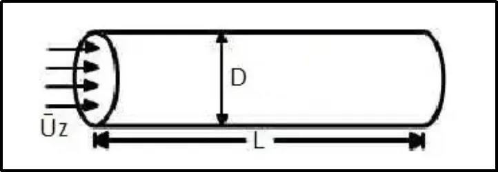
For flow in pipe of diameter D, experimental observations shows that for “fully developed” flow, laminar flow occurs when ReD">ReD < 2300. Therefore, let us, consider Re for flow is 2000. Assume diameter of pipe (D)=0.02m and length (L) = 2.5 m. also consider working fluid as water at temperature 25oC so the values of density (ρ">ρ)=997kg/m3">m3m3 and Dynamic Viscosity (μ">μ)=8.90X10⁻⁴Pa.sec.
FILE WRITING (in Matlab)
But, this time, we are going to create blockMeshDict file using Matlab coding by file parsing techniques. Prior, lest define all the given data first in our main program
Condition of working fluid according to problem statement.
Reynolds number (Re">Re) = 2000
Diameter of the pipe (D) = 0.02m
Length of the pipe (L) = 2.5m
Density of working fluid (ρ">ρ) = 997 kg/m3">m3m3
Dynamic viscosity of working fluid (μ">μ) = 8.9X10^-4 Pa.sec
%% Input parameters
% Reynold's Number
Re = 2000;
% Total Length of pipe(m)
L = 2.5;
% Diameter of pipe in meters
D = 0.02;
% Wedge Angle in degrees
th = input('<0> Wedge Angle in degrees - ');
% Density (kg/m^3)
rho = 997;
% Dynamic Viscosity (Pa.sec)
mu = 8.90e-4;
% Radius of pipe(m)
R = D/2;
Now, let us create separate function file to write blockMeshDict file in Matlab program. Create blockMeshDict file and start writing it using following ‘fopen’ command.
function[f1] = blockMesh(R,th,L,nx,ny,nz)

%% Writing BlockMeshDict file for openFoam
f1 = fopen('blockMeshDict','w');
Before defining any data we are going to state with printing header information in the form of comment which is not executable in OpenFoam
fprintf(f1,"/*--------------------------------*- C++ -*----------------------------------*n");
fprintf(f1,'  =========                 | n');
fprintf(f1,'  \      /  F ield         | OpenFOAM: The Open Source CFD Toolbox n');
fprintf(f1,'   \    /   O peration     | Website:  https://openfoam.org n');
fprintf(f1,'    \  /    A nd           | Version:  8 n');
fprintf(f1,'     \/     M anipulation  |n');
fprintf(f1,"*---------------------------------------------------------------------------*/n");
Next, we set units in meter, by converting all type of length in to meter.
fprintf(f1,'convertToMeters 1; n');Vertices:-
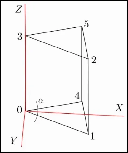
Afterward, in codes, we provide list of vertices by providing x,y,and z coordinates locations; its always start from vertex (0,0,0). so we have to create following geometry.
Mesh generation
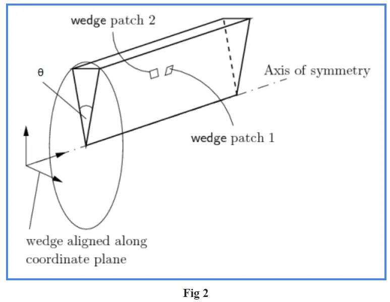
The mesh of the Pipe case includes a new feature: a block with fewer than 8 vertices will be used. There is an axi-symmetry in the case so it is not necessary to mesh the whole pipe but only a wedge of it. Since ∂∂θ=0">∂∂θ=0∂∂θ=0 for the whole domain, the results of the simulation will be the same while the number of elements of the mesh will be lower. Following figure represents a schematic view of the geometry that it is going to be created:
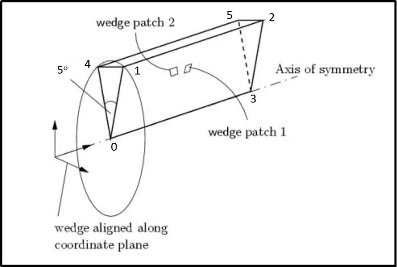
First of all, it is important to comprehend the collapsing of the vertices. It can be seen that vertices 0 and 3 are repeated in an adequate position within the parentheses to indicate that the two vertices that would be occupying this position have been collapsed.
Secondly, in the patches definition, the same vertices 0 and 3 are joined creating an empty patch forming the axis of the pipe. The patch type wedge is used in two faces to indicate that an axi-symmetry exists and there are no physical walls.
fprintf(f1,'vertices(n');
fprintf(f1,'    (0 0 0)n');
fprintf(f1,('    (%f %f 0)n'),R*cosd(th/2),R*sind(th/2));
fprintf(f1,('    (%f %f %f)n'),R*cosd(th/2),R*sind(th/2),L);
fprintf(f1,('    (%f 0 0)n'),L);
fprintf(f1,('    (%f %f 0)n'),R*cosd(th/2),-R*sind(th/2));
fprintf(f1,('    (%f %f %f)n);n'),R*cosd(th/2),-R*sind(th/2),L);
Next, we are going to define block for meshing. If we look at he mesh format first letter, in block parenthesis, is ‘hex’ which define type of mesh which is hexahedral mesh.
Then, again in parenthesis, we provide vertices number according to order which follow right hand thumb rule, meaning, thumb is the z axis and order of vertices follow rotational order of our other finger.
Then comes, number of mesh grid that we want to divide along x, y, and z length. We define it as (nx,ny,nz) format in main program.
Given mesh specification:
- Number of cells along the zdirection(longer dimension) = 500
- Number of cells along the longer xdirection = 20
- Number of cell for y direction =1
% Number of cells in x,y,z Directions
nx = 20;
ny = 1;
nz = 500;
Lastly, we give simple grading which is cell expansion ratios
Grading factor or expansion ratios:-
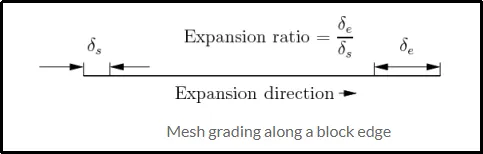
The expansion ratios enables the mesh to be graded, or refined, in specified directions. The ratio is that of the width of the end cell δe">δeδe along one edge of a block to the width of the start cell δs">δsδs along the edge as shown in below figure.
In simple format,
Expansion ratio = (size of end cell) / (size of starting cell)
The simple description specifies uniform expansion in the local x1">x1,x2">x2and x3">x3 directions respectively with only 3 expansion ratio. So here, we have 1 wedge shape block so we have to define hex mesh for 1 block.
There is a grading towards the wall to compute a more exact value of wall shear stress and towards the inlet where the flow is not fully developed and therefore the velocity profile changes.
fprintf(f1,('hex (0 4 1 0 3 5 2 3) (%d %d %d) simpleGrading (0.2 1 1)n);n'),nx,ny,nz);
In this case, for edge 4-1 and 5-2 we have radius curve so we will define this in edges section following way.
fprintf(f1,'edges(n');
fprintf(f1,'    arc 4 1 (0 %f 0)n',R);
fprintf(f1,'    arc 5 2 (%f %f 0)n);n',L,R);
Next, define boundary of the problem, in this we have to define faces of the our 3D block this should be in order according to right hand thumb rule. So set faces for this problem following way.
fprintf(f1,'boundary(n');
fprintf(f1,'     inletn');
fprintf(f1,'     {n');
fprintf(f1,'           type patch;n');
fprintf(f1,'           facesn');
fprintf(f1,'           (n');
fprintf(f1,'               (0 4 1 0)n');
fprintf(f1,'           );n');
fprintf(f1,'     }n');
fprintf(f1,'     outletn');
fprintf(f1,'     {n');
fprintf(f1,'           type patch;n');
fprintf(f1,'           facesn');
fprintf(f1,'           (n');
fprintf(f1,'               (3 5 2 3)n');
fprintf(f1,'           );n');
fprintf(f1,'     }n');
fprintf(f1,'     frontn');
fprintf(f1,'     {n');
fprintf(f1,'           type wedge;n');
fprintf(f1,'           facesn');
fprintf(f1,'           (n');
fprintf(f1,'               (0 1 2 3)n');
fprintf(f1,'           );n');
fprintf(f1,'     }n');
fprintf(f1,'     backn');
fprintf(f1,'     {n');
fprintf(f1,'           type wedge;n');
fprintf(f1,'           faces n');
fprintf(f1,'           (n');
fprintf(f1,'               (0 3 5 4)n');
fprintf(f1,'           );n');
fprintf(f1,'     }n');
fprintf(f1,'     pipewalln');
fprintf(f1,'     {n');
fprintf(f1,'           type wall;n');
fprintf(f1,'           facesn');
fprintf(f1,'           (n');
fprintf(f1,'               (1 4 5 2)n');
fprintf(f1,'           );n');
fprintf(f1,'     }n');
fprintf(f1,'     axisn');
fprintf(f1,'     {n');
fprintf(f1,'           type empty;n');
fprintf(f1,'           facesn');
fprintf(f1,'           (n');
fprintf(f1,'               (0 3 3 0)n');
fprintf(f1,'           );n');
fprintf(f1,'      }n');
fprintf(f1,');n');
fprintf(f1,'mergePatchPairsn');
fprintf(f1,'(n');
fprintf(f1,');n');
fprintf(f1,'// ************************************************************************* // n');
After running above codes, we will get our BlockMeshDict file as output.
/*--------------------------------*- C++ -*----------------------------------*
  =========                 |
        /  F ield         | OpenFOAM: The Open Source CFD Toolbox
       /   O peration     | Website:  https://openfoam.org
      /    A nd           | Version:  8
     /     M anipulation  |
*---------------------------------------------------------------------------*/
FoamFile
{
    version     2.0;
    format      ascii;
    class       dictionary;
    object      blockMeshDict;
}
// * * * * * * * * * * * * * * * * * * * * * * * * * * * * * * * * * * * * * //

convertToMeters 1;

vertices
(
    (0 0 0)
    (0.009990 0.000436 0)
    (0.009990 0.000436 2.500000)
    (0 0 2.500000)
    (0.009990 -0.000436 0)
    (0.009990 -0.000436 2.500000)
);

blocks
(
hex (0 4 1 0 3 5 2 3) (20 1 500) simpleGrading (0.2 1 1)
);

edges
(
    arc 4 1 (0 0.010000 0)
    arc 5 2 (2.500000 0.010000 0)
);

boundary
(
     inlet
     {
           type patch;
           faces
           (
               (0 4 1 0)
           );
     }
     outlet
     {
           type patch;
           faces
           (
               (3 5 2 3)
           );
     }
     front
     {
           type wedge;
           faces
           (
               (0 1 2 3)
           );
     }
     back
     {
           type wedge;
           faces
           (
               (0 3 5 4)
           );
     }
     pipewall
     {
           type wall;
           faces
           (
               (1 4 5 2)
           );
     }
     axis
     {
           type empty;
           faces
           (
               (0 3 3 0)
           );
      }
);

mergePatchPairs
(
);

// ************************************************************************* //
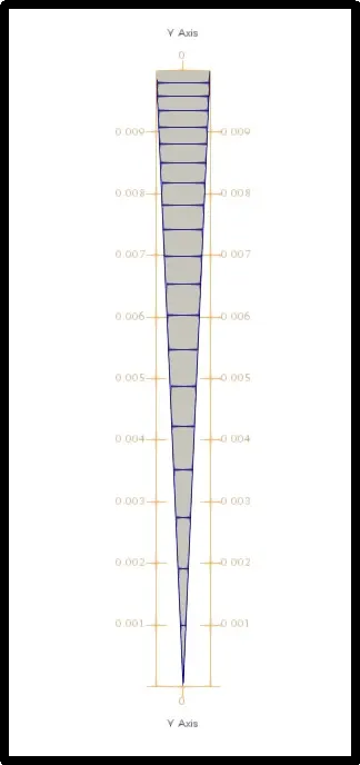
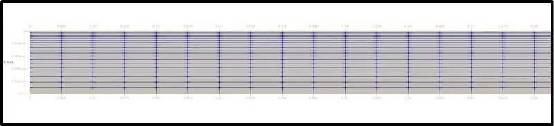
Copy above blockMeshDict file and replace it in the system directory of the pipe folder and by running this block mesh file we will get following mesh:
Furthermore, we are going to edit ‘controlDict’ file to provides time limits - start time and end time. Also to represent deltat. While selection of deltat CFL value shoud be less than 1. otherwise, the solution could stopped forcibly or it may diverge at the time of converging. So make following changes in ‘controlDict’ file.
/*--------------------------------*- C++ -*----------------------------------*
  =========                 |
        /  F ield         | OpenFOAM: The Open Source CFD Toolbox
       /   O peration     | Website:  https://openfoam.org
      /    A nd           | Version:  8
     /     M anipulation  |
*---------------------------------------------------------------------------*/
FoamFile
{
    version     2.0;
    format      ascii;
    class       dictionary;
    location    "system";
    object      controlDict;
}
// * * * * * * * * * * * * * * * * * * * * * * * * * * * * * * * * * * * * * //

application     icoFoam;

startFrom       startTime;

startTime       0;

stopAt          endTime;

endTime         2;

deltaT          0.0001;

writeControl    timeStep;

writeInterval   10;

purgeWrite      0;

writeFormat     ascii;

writePrecision  6;

writeCompression off;

timeFormat      general;

timePrecision   6;

runTimeModifiable true;


// ************************************************************************* //
Boundary and initial conditions
Then, we have to define initial value for pressure and velocity. In order to do that, we have to go back in cavity_copy directory using ‘cd ..’ command and select folder named ‘0’, which stand for initial values. In this case initial value for pressure and velocity.
When solving circulating internal flow, the most common boundary conditions are to fix an inlet velocity and an outlet pressure.
Initial setting for pressure
/*--------------------------------*- C++ -*----------------------------------*
  =========                 |
        /  F ield         | OpenFOAM: The Open Source CFD Toolbox
       /   O peration     | Website:  https://openfoam.org
      /    A nd           | Version:  8
     /     M anipulation  |
*---------------------------------------------------------------------------*/
FoamFile
{
    version     2.0;
    format      ascii;
    class       volScalarField;
    object      p;
}
// * * * * * * * * * * * * * * * * * * * * * * * * * * * * * * * * * * * * * //

dimensions      [0 2 -2 0 0 0 0];

internalField   uniform 0;

boundaryField
{
    inlet
    {
        type            zeroGradient;
    }

    outlet
    {
        type            fixedValue;
        value           uniform 0;
    }

    front
    {
        type            wedge;
    }

    back
    {
        type            wedge;
    }

    axis
    {
        type            empty;
    }

    pipewall
    {
        type            zeroGradient;
    }
}

// ************************************************************************* //
In the U dictionary one can find out a new type of boundary condition: inlet and outlet. It switches U and p between fixedValue and zeroGradient: the first when the flow is in-going and the second when it is outgoing.
Example: in circular pipe case, the outlet velocity will always be adapted to the conditions according to zeroGradient except if there is an inflow at the outlet patch. If this happens, to this inflow velocity it is assigned the value specified under the inletOutlet instruction and so the flow will always be outgoing.
Initial setting for Velocity
/*--------------------------------*- C++ -*----------------------------------*
  =========                 |
        /  F ield         | OpenFOAM: The Open Source CFD Toolbox
       /   O peration     | Website:  https://openfoam.org
      /    A nd           | Version:  8
     /     M anipulation  |
*---------------------------------------------------------------------------*/
FoamFile
{
    version     2.0;
    format      ascii;
    class       volVectorField;
    object      U;
}
// * * * * * * * * * * * * * * * * * * * * * * * * * * * * * * * * * * * * * //

dimensions      [0 1 -1 0 0 0 0];

internalField   uniform (0 0 0);

boundaryField
{
    inlet
    {
        type            fixedValue;
        value           uniform (0 0 0.1);
    }

    outlet
    {
        type            zeroGradient;
    }

    front
    {
        type            wedge;
    }

    back
    {
        type            wedge;
    }

    axis
    {
        type            empty;
    }

    pipewall
    {
        type            noSlip;
    }
}

// ************************************************************************* //
Next, we have to mention dynamic viscosity in transposeProperty in constant directory of the Pipe.
/*--------------------------------*- C++ -*----------------------------------*
  =========                 |
        /  F ield         | OpenFOAM: The Open Source CFD Toolbox
       /   O peration     | Website:  https://openfoam.org
      /    A nd           | Version:  8
     /     M anipulation  |
*---------------------------------------------------------------------------*/
FoamFile
{
    version     2.0;
    format      ascii;
    class       dictionary;
    location    "constant";
    object      transportProperties;
}
// * * * * * * * * * * * * * * * * * * * * * * * * * * * * * * * * * * * * * //

nu              [0 2 -1 0 0 0 0] 8.90e-4;


// ************************************************************************* //
Post-processing
Now, let us view the results in paraView by using ‘paraFoam’ command
RESULTS OF THE SIMULATION
The velocity at the inlet of the pipe (non-developed flow)
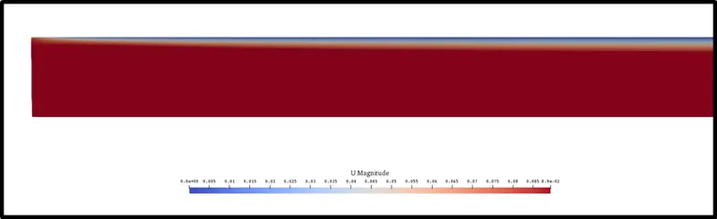
In above figure we can notice that the shear stress along wall surface is starting to increase as fluid moving forward.
The velocity field at the outlet of the pipe (developed flow)
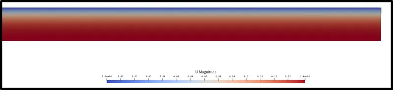
And at the end of the pipe, we can see, developed wall shear stress and velocity remain stable.
Mirroring the results in paraview
The laminar flow through a symmetrically circular pipe. In this problem, the streamlines travel on a straight line and the flow-pattern is identical in every plane that passes through the central axis of the pipe referred to as the symmetry axis. Such a flow is called an axisymmetric flow. The flow pattern for the mentioned problem is shown below in Fig 1.
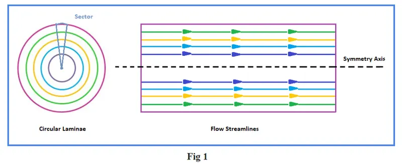
In the above figure, the concentric circles represent the fluid laminae and the fluid properties will be the same along each circular lamina for an axisymmetric flow. These fluid properties might vary with the flow distance but the symmetricity will not change. The flow streamlines on either side of the symmetry axis will remain a mirror image of one another. So it is sufficient to perform a 2D simulation for a sector (of small angle) across the flow distance as shown in Fig 2 below.
Simulating for a small sector will just simulate for one half of the flow in the diametral plane that stretches across the flow distance. One might want to view the complete solution for the entire flow in the diametral plane. This can be done by reflecting the half solution across the symmetry axis/plane. In Paraview, the Reflect filter can be used for this purpose. The procedure to reflect the result about any plane in Paraview is mentioned below.
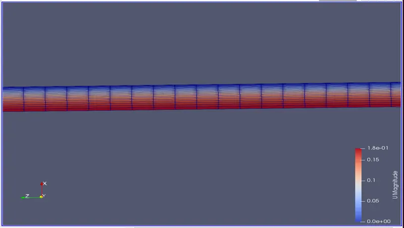
Results before mirroring
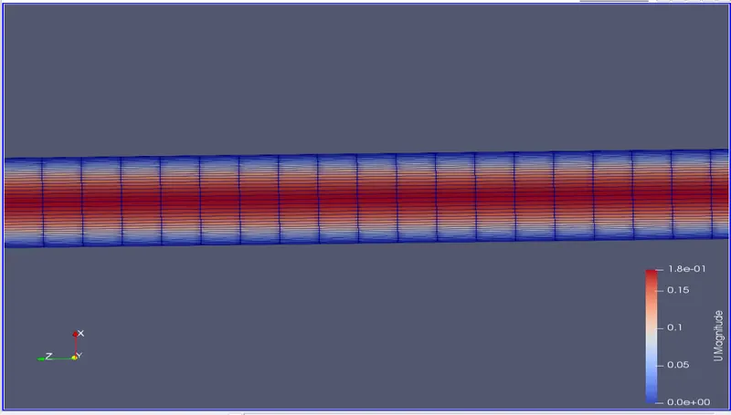
Results after mirroring
Velocity profile after the entrance length by using the plot over line
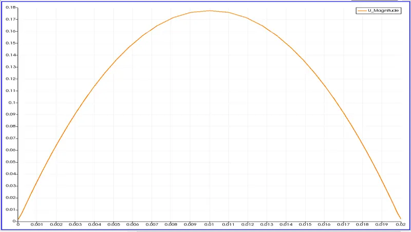
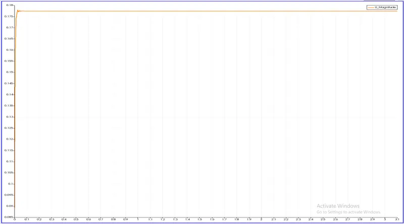
velocity prfile at length 2.5m `v_(max) = 0.177`
Computing the gradients for U-magnitude using
Now, Press ‘Ctrl+space’ or click Filters -> search in paraview. A search widow will pop up for the mentioned filter. Type gradient of Unstructured Data set and select it.
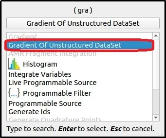
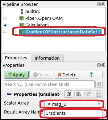
The property window changes as follows. Select scalar array as mag_u i.e. magnitude of velocity and give required result array name and click apply which will give us a gradient of the magnitude of velocity.
Compute the shear-stress quantity
Shear stress formula is given as
`tau=(4*mu*v_(avg))/(R)`Tau=μdudy">
Where,
μ">μ is Dynamic viscosity
τ">τ is Shear stress
R is radius
Therefore, we can obtain shear stress by multiplying the velocity gradient with the dynamic viscosity of the fluid under study.
So, in this project, we have considered the water as working fluid at 25oC room temperature which dynamic viscosity is 8.90e-4 N/m2">m2m2.
Then, again click on the Calculator tool and same way create tau array using product of velocity gradient and dynamic viscosity.
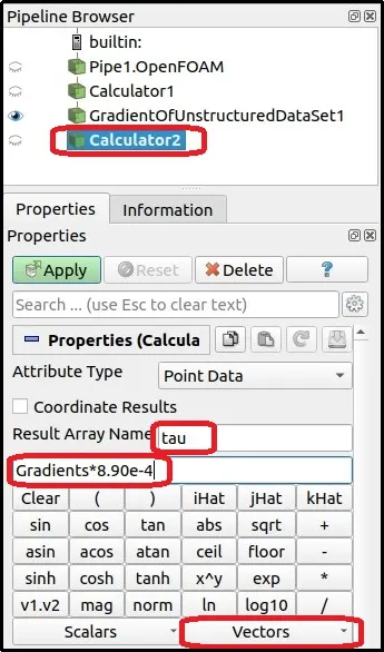
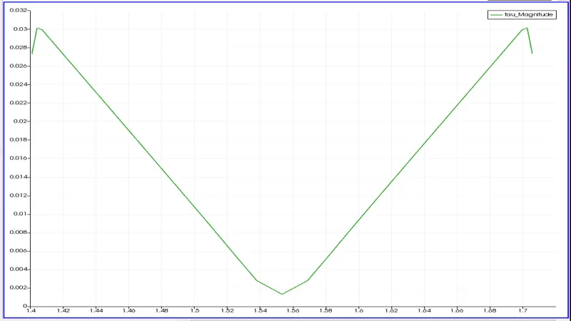
After plotting shear stress we will get following plot as our result `tau = 0.0301`
Hydro-dynamic length
Flow at the entrance to a pipe
Consider a flow entering a pipe. Let us think of the entering flow being uniform, so inviscid. As soon as the flow 'hits' the pipe many changes take place. The most important of these is that viscosity imposes itself on the flow and the "No Slip" condition at the wall of the pipe comes into effect. Consequently the velocity components are each zero on the wall, ie., u = v = 0. The flow adjacent to the wall decelerates continuously. We have a layer close to the body where the velocity builds up slowly from zero at wall to a uniform velocity towards the center of the pipe. This layer is what is called the Boundary Layer. Viscous effects are dominant within the boundary layer. Outside of this layer is the inviscid core where viscous effects are negligible or absent.
The boundary layer is not a static phenomenon; it is dynamic. it grows meaning that its thickness increases as we move downstream. From Fig. it is seen that the boundary layer from the walls grows to such an extent that they all merge on the centreline of the pipe. Once this takes place, inviscid core terminates and the flow is all viscous. The flow is now called a Fully Developed Flow. The velocity profile becomes parabolic. Once the flow is fully developed the velocity profile does not vary in the flow direction. In fact in this region the pressure gradient and the shear stress in the flow are in balance. The length of the pipe between the start and the point where the fully developed flow begins is called the Entrance Length. Denoted by Le, the entrance length is a function of the Reynolds Number of the flow. In general,
`l_e/D=0.06*R_e` for laminar flow
`l_e/D=4.4*R_e^((1)/(6))` for turbulent flow
At critical condition, i.e., Red =2300, the Le/d for a laminar flow is 138. Under turbulent conditions it ranges from 18(at Red = 4000) to 95 (at Red=108)
Application decides whether a long enough entrance length is required or a shorter one is required. Take wind tunnel for instance. Here the aim is to have a uniform flow over the model in the test section. So one desires to have a longer entrance length.
By using the plot over line we will be plotting the line along the length of the pipe and calculating the velocity along the line as shown in the below fig
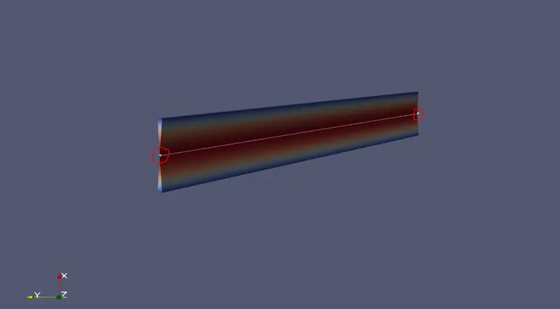
when ever the maximum velocity remain constant the entrence length will end
ANALYTICAL CALCULATIONS
Average Velocity:-
`V_(avg)=(R_eμ)/(ρD)`
% Average Velcity
V_avg = (Re*mu)/(rho*D);
`v_(avg) = 0.0937`
Maximum velocity:-
`v_(max)=2*v_(avg)`
`v_(max)=2*0.0937`
`v_(max)=0.1874`
Pressure drop across the length of pipe:-
`ΔP=(32μLV_(avg))/(D^2)`
length L = 0.5
`Deltap = 3.5`
Wall Shear stress
`tau_w=(4*mu*v_(avg))/(R)`
`tau_w=0.0356`
Velocity at various radius(r) near fully developed flow region
`V_r=2*V_(avg)(1−(r^2)/(R^2))`
% ANALYTICAL
R = 0.01;
r=linspace(-R,R,1000);

V_avg = (Re*mu)/(rho*D);

% Velocity_analytical
V_A=2*V_avg*(1-(r.^2/R^2));
Analytical Hydro-dynamic length
`l_e/D=0.06*R_e`
`l_e = 2.52`
where
`l_e` entrance length'
D Diameter
`R_e` renolds number
Comparing the NUMERICAL AND ANALYTICAL CALCULATIONS
comparing the velocity profile using MATLAB
clear all
close all
clc


% Reynold's Number
Re = 2100;
% Total Length of pipe(m)
L = 3.1;
% Diameter of pipe in meters
D = 0.02;
% Density (kg/m^3)
rho = 997;
% Dynamic Viscosity (Pa.sec)
mu = 8.90e-4;
% Radius of pipe(m)
R = D/2;

% ANALYTICAL
R = 0.01;
r=linspace(-R,R,1000);

V_avg = (Re*mu)/(rho*D);

% Velocity_analytical
V_A=2*V_avg*(1-(r.^2/R^2));


%NUMERICAL

v_r = csvread("v_p.csv",1,1);
c = csvread("v_p.csv",1);


for i = 1:1000

    %velocity_numerical
    V_n(i) = v_r(i)* (1-(c(i)^2));

end


figure(1)
plot(r,V_A,'r','linewidth',1)
hold on
plot(r,V_n,'--','color','k','linewidth',2.5)
xlabel('<---- Radius of pipe in m ---->','fontweight','bold','fontsize',14)
ylabel(' Velocity in m/s ------>','fontweight','bold','fontsize',14)
legend(' Analytical method',' Numerical method')
grid on
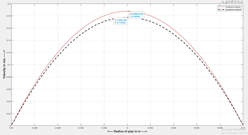
Below graph shows the velocity profile comparison between NUMERICAL AND ANALYTICAL
Validate Hydro-dynamic length with the numerical result
ANALYTICAL value is 2.52 m
NUMERICAL value is 0.08 m
| ANALYTICAL | NUMERICAL | |
| `v_(max)` | 0.1875 | 0.177416 |
| `Deltap` for length 0.5m | 3.5 | 3.8185 |
| `tau_w` | 0.0356 | 0.0301 |
We can see that the values of the ANALYTICAL and NUMERICAL are vary because there will be a numerical error in the internal calculations so there will be a change in the values by comparing the both
complete code of the blockmeshdict
function[f1] = blockMesh(R,th,L,nx,ny,nz)

%% Writing BlockMeshDict file for openFoam
f1 = fopen('blockMeshDict','w');

%% Input parameters
% Reynold's Number
Re = 2100;
% Total Length of pipe(m)
L = 3.1;
% Diameter of pipe in meters
D = 0.02;
% Wedge Angle in degrees
th = input('<0> Wedge Angle in degrees - ');
% Density (kg/m^3)
rho = 997;
% Dynamic Viscosity (Pa.sec)
mu = 8.90e-4;
% Radius of pipe(m)
R = D/2;
% Number of cells in x,y,z Directions
nx = 20;
ny = 1;
nz = 500;

fprintf(f1,"/*--------------------------------*- C++ -*----------------------------------*n");
fprintf(f1,'  =========                 | n');
fprintf(f1,'  \      /  F ield         | OpenFOAM: The Open Source CFD Toolbox n');
fprintf(f1,'   \    /   O peration     | Website:  https://openfoam.org n');
fprintf(f1,'    \  /    A nd           | Version:  8 n');
fprintf(f1,'     \/     M anipulation  |n');
fprintf(f1,"*---------------------------------------------------------------------------*/n");
fprintf(f1,'FoamFile n');
fprintf(f1,'{ n');
fprintf(f1,'    version     2.0;n');
fprintf(f1,'    format      ascii;n');
fprintf(f1,'    class       dictionary;n');
fprintf(f1,'    object      blockMeshDict;n');
fprintf(f1,'} n');
fprintf(f1,'// * * * * * * * * * * * * * * * * * * * * * * * * * * * * * * * * * * * * *// n');
fprintf(f1,'convertToMeters 1; n');
fprintf(f1,'vertices(n');
fprintf(f1,'    (0 0 0)n');
fprintf(f1,('    (%f %f 0)n'),R*cosd(th/2),R*sind(th/2));
fprintf(f1,('    (%f %f %f)n'),R*cosd(th/2),R*sind(th/2),L);
fprintf(f1,('    (%f 0 0)n'),L);
fprintf(f1,('    (%f %f 0)n'),R*cosd(th/2),-R*sind(th/2));
fprintf(f1,('    (%f %f %f)n);n'),R*cosd(th/2),-R*sind(th/2),L);
fprintf(f1,'blocks(n');
fprintf(f1,('hex (0 4 1 0 3 5 2 3) (%d %d %d) simpleGrading (0.2 1 1)n);n'),nx,ny,nz);
fprintf(f1,'edges(n');
fprintf(f1,'    arc 4 1 (0 %f 0)n',R);
fprintf(f1,'    arc 5 2 (%f %f 0)n);n',L,R);
fprintf(f1,'boundary(n');
fprintf(f1,'     inletn');
fprintf(f1,'     {n');
fprintf(f1,'           type patch;n');
fprintf(f1,'           facesn');
fprintf(f1,'           (n');
fprintf(f1,'               (0 4 1 0)n');
fprintf(f1,'           );n');
fprintf(f1,'     }n');
fprintf(f1,'     outletn');
fprintf(f1,'     {n');
fprintf(f1,'           type patch;n');
fprintf(f1,'           facesn');
fprintf(f1,'           (n');
fprintf(f1,'               (3 5 2 3)n');
fprintf(f1,'           );n');
fprintf(f1,'     }n');
fprintf(f1,'     frontn');
fprintf(f1,'     {n');
fprintf(f1,'           type wedge;n');
fprintf(f1,'           facesn');
fprintf(f1,'           (n');
fprintf(f1,'               (0 1 2 3)n');
fprintf(f1,'           );n');
fprintf(f1,'     }n');
fprintf(f1,'     backn');
fprintf(f1,'     {n');
fprintf(f1,'           type wedge;n');
fprintf(f1,'           faces n');
fprintf(f1,'           (n');
fprintf(f1,'               (0 3 5 4)n');
fprintf(f1,'           );n');
fprintf(f1,'     }n');
fprintf(f1,'     pipewalln');
fprintf(f1,'     {n');
fprintf(f1,'           type wall;n');
fprintf(f1,'           facesn');
fprintf(f1,'           (n');
fprintf(f1,'               (1 4 5 2)n');
fprintf(f1,'           );n');
fprintf(f1,'     }n');
fprintf(f1,'     axisn');
fprintf(f1,'     {n');
fprintf(f1,'           type empty;n');
fprintf(f1,'           facesn');
fprintf(f1,'           (n');
fprintf(f1,'               (0 3 3 0)n');
fprintf(f1,'           );n');
fprintf(f1,'      }n');
fprintf(f1,');n');
fprintf(f1,'mergePatchPairsn');
fprintf(f1,'(n');
fprintf(f1,');n');
fprintf(f1,'// ************************************************************************* // n');
fclose(f1);


end