Simulation of Flow through a pipe in OpenFoam
OBJECTIVE:
- To simulate an axi-symmetric flow by applying the wedge boundary condition. The flow is laminar and flows through a constant cross-section pipe at an inlet Reynold's number of 2100. we can do a transient or steady state simulation and will validate results with the Hagen- Poiseuille's equations for the fully developed flow.
- To write a code in Matlab to automate the generation of blockMeshDict file. The code should take inputs like pipe length, diameter, wedge angle, etc and output a fully functional blockMeshDict file.
Expected Results
- Validate Hydro-dynamic length with the numerical result
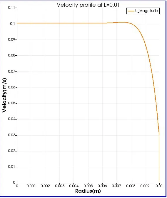
- Validate the fully developed flow velocity profile with its analytical profile
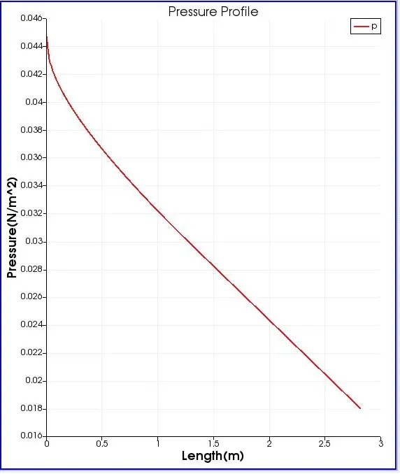
- Validate maximum velocity and pressured drop for fully developed flow
- Post-process Shear stress and validate wall shear stress for fully developed flow
Solutions:
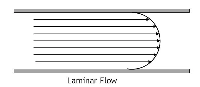
Laminar flow, type of fluid (gas or liquid) flow in which the fluid travels smoothly or in regular paths, in contrast to turbulent flow, in which the fluid undergoes irregular fluctuations and mixing. In laminar flow, sometimes called streamline flow, the velocity, pressure, and other flow properties at each point in the fluid remain constant. Laminar flow over a horizontal surface may be thought of as consisting of thin layers, or laminae, all parallel to each other. The fluid in contact with the horizontal surface is stationary, but all the other layers slide over each other. A deck of new cards, as a rough analogy, may be made to “flow” laminarly.
Laminar flow in a straight pipe may be considered as the relative motion of a set of concentric cylinders of fluid, the outside one fixed at the pipe wall and the others moving at increasing speeds as the center of the pipe is approached. Smoke rising in a straight path from a cigarette is undergoing laminar flow. After rising a small distance, the smoke usually changes to turbulent flow, as it eddies and swirls from its regular path.
Laminar flow is common only in cases in which the flow channel is relatively small, the fluid is moving slowly, and its viscosity is relatively high. Oil flow through a thin tube or blood flow through capillaries is laminar. Most other kinds of fluid flow are turbulent except near solid boundaries, where the flow is often laminar, especially in a thin layer just adjacent to the surface. See fluid mechanics.
Hydrodynamic entrance length:
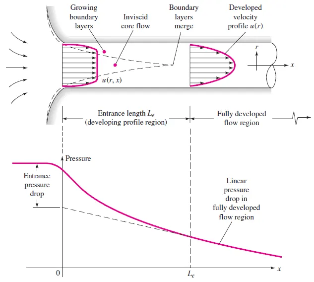
For internal flow regime an entrance region is typical. In this region a nearly inviscid upstream flow converges and enters the tube. To characterize this region the hydrodynamic entrance length is introduced and is approximately equal to:

The maximum hydrodynamic entrance length, at ReD,crit = 2300 (laminar flow), is Le = 138d, where D is the diameter of the pipe. This is the longest development length possible. In turbulent flow, the boundary layers grow faster, and Le is relatively shorter. For any given problem, Le / D has to be checked to see if Le is negligible when compared to the pipe length. At a finite distance from the entrance, the entrance effects may be neglected, because the boundary layers merge and the inviscid core disappears. The tube flow is then fully developed.
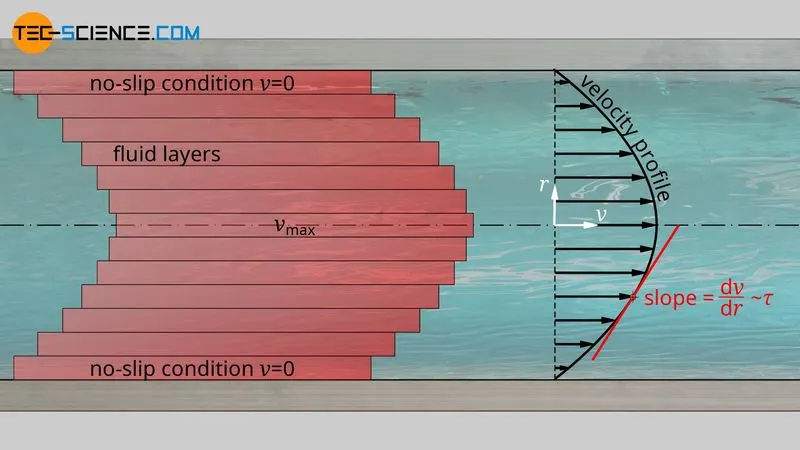
In principle, the speed of the flow within the pipe is not constant over the cross-section. There is friction between the fluid and the pipe, which is why the flow velocity near the wall is lower than in the middle of the pipe. At the wall, the fluid even adheres to the wall due to the adhesive forces. Thus, there is no relative speed between fluid and wall. This is also called the no-slip condition. But the individual fluid layers also have friction between each other due to the viscosity of the fluid. This leads to the formation of a certain velocity profile, the course of which is yet to be determined. It should be noted, however, that the flow velocity is maximum in the middle of the pipe and then drops to zero as far as the wall.
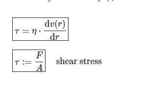
The flow resistance to be overcome, which is necessary to shear the individual fluid layers against each other, depends on the viscosityof the fluid. The flow resistance is expressed by the shear stress τ, i.e. as the force per unit area required to move a fluid layer. This shear stress depends on how much the fluid layers are displaced against each other. This in turn is expressed by the velocity gradient perpendicular to the flow direction, i.e. by the slope of the velocity profile in the radial direction dv(r)/dr (also called shear rate). The mathematical relationship between the two quantities is described by the viscosity η (Newton’s law of fluid motion):
Mean flow velocity
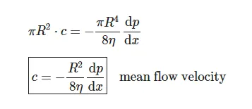
With its parabolic velocity profile, a flow inside a pipe has no characteristic velocity in principle. Therefore, a mean flow velocity c is often defined to characterize such flows. The mean flow velocity is defined as a constant velocity over the entire cross-section which provides the same flow rate as the real velocity profile. With A=π⋅R2 as the inner pipe cross-section, the mean flow velocity c can be determined by the volume flow rate V*

In the above derivation, it was used that the quotient of traveled distance Δx and time Δt just corresponds to the mean flow velocity. Equating the equations finally provides the mean flow velocity
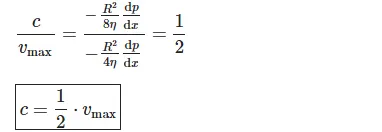
The following relationship applies between the maximum flow velocity Vmax and the mean flow velocity
Pressure loss
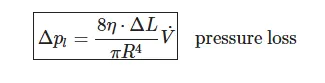
As already explained, the pressure gradient dp/dx in the upper equations represents the drive for the flow of the fluid. According to the equation, this directly influences the flow rate. Conversely, this means that a pressure gradient must exist for the desired flow rate. This requires a pump that ultimately generates this pressure gradient (at this point the negative sign is omitted since only the amounts are decisive anyway)
For a friction-free flow, on the other hand, no such pressure drop would have to be applied in the steady-state to keep the fluid flowing. Once set in motion, the fluid would flow through the pipe without loss of speed. The application of the pressure is therefore due to the friction loss, which is equivalent to a pressure drop. In the steady case, the pressure created by a pump must fully compensate for the pressure loss in order to keep the fluid flowing. The above formula is therefore equivalent to the pressure loss Δpl, which occurs over the pipe length ΔL:
Now the following calculation are done for analytical solutions of the Hagen Poiseuille law.
- Reynolds Number = 2100
- Kinematuc viscosity = 1e-6
- Dynamic Viscosity = 0.00089 N-s/m2
- Density of water = 1000Kg/m3
- Diameter of pipe = 20mm
- Hydrodynamic length Le = 00.06ReD = 2.53m
- Average velocity Vavg = Re*v/D
= 0.09345ms-1
- Maximum velocity Vmax = 2Vavg
0.01869ms-1
- Pressure
p = 8VavgmuL/R2 = 18.763Nm-2
In OpenFOAM, we have to provide the pressure boundary condition in terms of kinematic pressure and for that to begin we are going to write code to develop a Block mesh file for OpenFOAM to execute.
Pk = DeltaP/p
= 0.018m2s-2
MATLAB CODE:
clear all
close all
clc

% The Reynolds number
Re = 2100
% The Diameter of pipe
D = 0.004
% The Entry length of pipe
L =0.06*Re*D
% The total length of pipe
L_p = L+0.7
% Radius of pipe
r = D/2
% Angle of wedge (less than 5)
theta = 4
% Dynamic viscosity
mu = 0.89e-3
% Density
rho = 997

% Hagen poiseuille flow equations
v_avg = (Re*mu)/(rho*D)
v_max = 2*(v_avg)
del_p = (8*mu*L_p*v_avg)/(r^2)
kinematic_p = del_p/rho

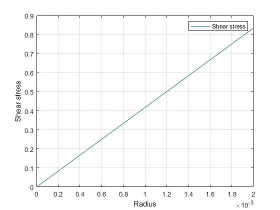
% calculating shear stress
R = linspace(0,(D/2),1000)

for i = 1:length(R)
    tau(i) = 2*mu*v_max*(abs(R(i)))/r^2
end

plot(R,tau)
xlabel('Radius')
ylabel('Shear stress')
grid on
legend ('Shear stress')- The inputs are provided and stored withe the resspective matlab variables such as reynolds number,Diameter,Radius of pipe etc..
- The hagen poiseulle flow equations is stored with maximum and average velocity equation and the kinematic pressure is also solved for obatining the equation.
- The shear stress is valucualted usimg the Radius amd for loop for different radius terms.
- Plot is taken with r and tau following the labels and legend.
header1='/*----------------------------------*- C++ -*------------------------------------*'
header2='  =========                 |                                                    '
header3='   \      /  F ield                | OpenFOAM: The Open Source CFD Toolbox      '
header4='    \    /   O peration        | Website:  https://openfoam.org                 '
header5='     \  /    A nd                 | Version:  7                                 '
header6='      \/     M anipulation   |                                                  '
header7='*----------------------------------------------------------------------------------*/'

f1 = fopen('blockMeshDict','w')
fprintf(f1, '%sn', header1)
fprintf(f1, '%sn', header2)
fprintf(f1, '%sn', header3)
fprintf(f1, '%sn', header4)
fprintf(f1, '%sn', header5)
fprintf(f1, '%sn', header6)
fprintf(f1, '%sn', header7)

fprintf(f1, 'FoamFilen{n')
fprintf(f1, '%12s t 2.0;n','version')
fprintf(f1, '%12s t ascii;n','format')
fprintf(f1, '%12s t dictionary;n','class')
fprintf(f1, '%12s t blockMeshDict;n','object')
fprintf(f1, '}n')
header8='// * * * * * * * * * * * * * * * * * * * * * * * * * * * * * * * * * * * * * //'
fprintf(f1, '%snn',header8)


fprintf(f1, 'convertToMeters 1;nn')

fprintf(f1, 'verticesn')
fprintf(f1, '(n')
fprintf(f1, 't (%d  %d %d)n',0,0,0)
fprintf(f1, 't (%d  %d %d)n',0,r*cosd(theta/2),r*sind(theta/2))
fprintf(f1, 't (%d  %d %d)n',0,r*cosd(theta/2),-r*sind(theta/2))
fprintf(f1, 't (%d  %d %d)n',L_p,0,0)
fprintf(f1, 't (%d  %d %d)n',L_p,r*cosd(theta/2),r*sind(theta/2))
fprintf(f1, 't (%d  %d %d)n',L_p,r*cosd(theta/2),-r*sind(theta/2))
fprintf(f1, ');nn')


fprintf(f1, 'blocksn')
fprintf(f1, '(n')
fprintf(f1, 't hex (0 3 5 2 0 3 4 1) (%d %d %d)',300,30,1)
fprintf(f1, ' SimpleGrading (1 0.1 1)nn')
fprintf(f1, ');nn')

fprintf(f1, 'edgesn')
fprintf(f1, '(n')
fprintf(f1, 't arc %d %d (%d %d %d)n',1,2,0,r,0)
fprintf(f1, 't arc %d %d (%d %d %d)n',4,5,L_p,r,0)
fprintf(f1, ');nn')

fprintf(f1, 'boundaryn')
fprintf(f1, '(n')
fprintf(f1, 't inlet n')
fprintf(f1, 't {n')
fprintf(f1, 'tt type patch;n')
fprintf(f1, 'tt facesn')
fprintf(f1, 'tt (n')
fprintf(f1, 'ttt (0 1 2 0)n')
fprintf(f1, 'tt );n')
fprintf(f1, 't }n')


fprintf(f1, 't outletn')
fprintf(f1, 't {n')
fprintf(f1, 'tt type patch;n')
fprintf(f1, 'tt facesn')
fprintf(f1, 'tt (n')
fprintf(f1, 'ttt (3 5 4 3)n')
fprintf(f1, 'tt );n')
fprintf(f1, 't }n')


fprintf(f1, 't topn')
fprintf(f1, 't {n')
fprintf(f1, 'tt type wall;n')
fprintf(f1, 'tt facesn')
fprintf(f1, 'tt (n')
fprintf(f1, 'ttt (1 4 5 2)n')
fprintf(f1, 'tt );n')
fprintf(f1, 't }n')

fprintf(f1, 't frontn')
fprintf(f1, 't {n')
fprintf(f1, 'tt type wedge;n')
fprintf(f1, 'tt facesn')
fprintf(f1, 'tt (n')
fprintf(f1, 'ttt (0 3 4 1)n')
fprintf(f1, 'tt );n')
fprintf(f1, 't }n')

fprintf(f1, 't backn')
fprintf(f1, 't {n')
fprintf(f1, 'tt type wedge;n')
fprintf(f1, 'tt facesn')
fprintf(f1, 'tt (n')
fprintf(f1, 'ttt (0 2 5 3)n')
fprintf(f1, 'tt );n')
fprintf(f1, 't }n')

fprintf(f1, 't axisn')
fprintf(f1, 't {n')
fprintf(f1, 'tt type empty;n')
fprintf(f1, 'tt facesn')
fprintf(f1, 'tt (n')
fprintf(f1, 'ttt (0 3 3 0)n')
fprintf(f1, 'tt );n')
fprintf(f1, 't }n')
fprintf(f1, '); nn')

fprintf(f1, 'mergePatchPairsn')
fprintf(f1, '(n')
fprintf(f1, ');n')

header9='// * * * * * * * * * * * * * * * * * * * * * * * * * * * * * * * * * * * * * //'
fprintf(f1, '%sn',header9)

fclose(f1)- Now using the file parsing method the blockMesh C format text is excecuted using the above codes
- The structure has to be similar as a typicl blockMesh dict file.
- The f print f command is used to print the particular line in the text file and stored and then finally closed with f close f1.
FULLCODE:
clear all
close all
clc

% The Reynolds number
Re = 2100
% The Diameter of pipe
D = 0.004
% The Entry length of pipe
L =0.06*Re*D
% The total length of pipe
L_p = L+0.7
% Radius of pipe
r = D/2
% Angle of wedge (less than 5)
theta = 4
% Dynamic viscosity
mu = 0.89e-3
% Density
rho = 997

% Hagen poiseuille flow equations
v_avg = (Re*mu)/(rho*D)
v_max = 2*(v_avg)
del_p = (8*mu*L_p*v_avg)/(r^2)
kinematic_p = del_p/rho

% calculating shear stress
R = linspace(0,(D/2),1000)

for i = 1:length(R)
    tau(i) = 2*mu*v_max*(abs(R(i)))/r^2
end

plot(R,tau)
xlabel('Radius')
ylabel('Shear stress')
grid on
legend ('Shear stress')
header1='/*----------------------------------*- C++ -*------------------------------------*'
header2='  =========                 |                                                    '
header3='   \      /  F ield                | OpenFOAM: The Open Source CFD Toolbox      '
header4='    \    /   O peration        | Website:  https://openfoam.org                 '
header5='     \  /    A nd                 | Version:  7                                 '
header6='      \/     M anipulation   |                                                  '
header7='*----------------------------------------------------------------------------------*/'

f1 = fopen('blockMeshDict','w')
fprintf(f1, '%sn', header1)
fprintf(f1, '%sn', header2)
fprintf(f1, '%sn', header3)
fprintf(f1, '%sn', header4)
fprintf(f1, '%sn', header5)
fprintf(f1, '%sn', header6)
fprintf(f1, '%sn', header7)

fprintf(f1, 'FoamFilen{n')
fprintf(f1, '%12s t 2.0;n','version')
fprintf(f1, '%12s t ascii;n','format')
fprintf(f1, '%12s t dictionary;n','class')
fprintf(f1, '%12s t blockMeshDict;n','object')
fprintf(f1, '}n')
header8='// * * * * * * * * * * * * * * * * * * * * * * * * * * * * * * * * * * * * * //'
fprintf(f1, '%snn',header8)


fprintf(f1, 'convertToMeters 1;nn')

fprintf(f1, 'verticesn')
fprintf(f1, '(n')
fprintf(f1, 't (%d  %d %d)n',0,0,0)
fprintf(f1, 't (%d  %d %d)n',0,r*cosd(theta/2),r*sind(theta/2))
fprintf(f1, 't (%d  %d %d)n',0,r*cosd(theta/2),-r*sind(theta/2))
fprintf(f1, 't (%d  %d %d)n',L_p,0,0)
fprintf(f1, 't (%d  %d %d)n',L_p,r*cosd(theta/2),r*sind(theta/2))
fprintf(f1, 't (%d  %d %d)n',L_p,r*cosd(theta/2),-r*sind(theta/2))
fprintf(f1, ');nn')


fprintf(f1, 'blocksn')
fprintf(f1, '(n')
fprintf(f1, 't hex (0 3 5 2 0 3 4 1) (%d %d %d)',300,30,1)
fprintf(f1, ' SimpleGrading (1 0.1 1)nn')
fprintf(f1, ');nn')

fprintf(f1, 'edgesn')
fprintf(f1, '(n')
fprintf(f1, 't arc %d %d (%d %d %d)n',1,2,0,r,0)
fprintf(f1, 't arc %d %d (%d %d %d)n',4,5,L_p,r,0)
fprintf(f1, ');nn')

fprintf(f1, 'boundaryn')
fprintf(f1, '(n')
fprintf(f1, 't inlet n')
fprintf(f1, 't {n')
fprintf(f1, 'tt type patch;n')
fprintf(f1, 'tt facesn')
fprintf(f1, 'tt (n')
fprintf(f1, 'ttt (0 1 2 0)n')
fprintf(f1, 'tt );n')
fprintf(f1, 't }n')


fprintf(f1, 't outletn')
fprintf(f1, 't {n')
fprintf(f1, 'tt type patch;n')
fprintf(f1, 'tt facesn')
fprintf(f1, 'tt (n')
fprintf(f1, 'ttt (3 5 4 3)n')
fprintf(f1, 'tt );n')
fprintf(f1, 't }n')


fprintf(f1, 't topn')
fprintf(f1, 't {n')
fprintf(f1, 'tt type wall;n')
fprintf(f1, 'tt facesn')
fprintf(f1, 'tt (n')
fprintf(f1, 'ttt (1 4 5 2)n')
fprintf(f1, 'tt );n')
fprintf(f1, 't }n')

fprintf(f1, 't frontn')
fprintf(f1, 't {n')
fprintf(f1, 'tt type wedge;n')
fprintf(f1, 'tt facesn')
fprintf(f1, 'tt (n')
fprintf(f1, 'ttt (0 3 4 1)n')
fprintf(f1, 'tt );n')
fprintf(f1, 't }n')

fprintf(f1, 't backn')
fprintf(f1, 't {n')
fprintf(f1, 'tt type wedge;n')
fprintf(f1, 'tt facesn')
fprintf(f1, 'tt (n')
fprintf(f1, 'ttt (0 2 5 3)n')
fprintf(f1, 'tt );n')
fprintf(f1, 't }n')

fprintf(f1, 't axisn')
fprintf(f1, 't {n')
fprintf(f1, 'tt type empty;n')
fprintf(f1, 'tt facesn')
fprintf(f1, 'tt (n')
fprintf(f1, 'ttt (0 3 3 0)n')
fprintf(f1, 'tt );n')
fprintf(f1, 't }n')
fprintf(f1, '); nn')

fprintf(f1, 'mergePatchPairsn')
fprintf(f1, '(n')
fprintf(f1, ');n')

header9='// * * * * * * * * * * * * * * * * * * * * * * * * * * * * * * * * * * * * * //'
fprintf(f1, '%sn',header9)

fclose(f1)
BlockMeshDict:
/*--------------------------------*- C++ -*----------------------------------*
  =========                 |
  \      /  F ield         | OpenFOAM: The Open Source CFD Toolbox
   \    /   O peration     | Website:  https://openfoam.org
    \  /    A nd           | Version:  7
     \/     M anipulation  |
*---------------------------------------------------------------------------*/
FoamFile
{
    version     2.0;
    format      ascii;
    class       dictionary;
    object      blockMeshDict;
}
// * * * * * * * * * * * * * * * * * * * * * * * * * * * * * * * * * * * * * //

convertToMeters 1;

vertices
(
	 (0  0 0)
	 (0  1.998782e-03 6.979899e-05)
	 (0  1.998782e-03 -6.979899e-05)
	 (1.204000e+00  0 0)
	 (1.204000e+00  1.998782e-03 6.979899e-05)
	 (1.204000e+00  1.998782e-03 -6.979899e-05)
);

blocks
(
	 hex (0 3 5 2 0 3 4 1) (300 30 1) SimpleGrading (1 0.1 1)

);

edges
(
	 arc 1 2 (0 2.000000e-03 0)
	 arc 4 5 (1.204000e+00 2.000000e-03 0)
);

boundary
(
	 inlet
	 {
		 type patch;
		 faces
		 (
			 (0 1 2 0)
		 );
	 }
	 outlet
	 {
		 type patch;
		 faces
		 (
			 (3 5 4 3)
		 );
	 }
	 top
	 {
		 type wall;
		 faces
		 (
			 (1 4 5 2)
		 );
	 }
	 front
	 {
		 type wedge;
		 faces
		 (
			 (0 3 4 1)
		 );
	 }
	 back
	 {
		 type wedge;
		 faces
		 (
			 (0 2 5 3)
		 );
	 }
	 axis
	 {
		 type empty;
		 faces
		 (
			 (0 3 3 0)
		 );
	 }
);

mergePatchPairs
(
);
// * * * * * * * * * * * * * * * * * * * * * * * * * * * * * * * * * * * * * //- After excecuting the above matlab code the blockMesh looks like this the original block mesh is replaced with this one which can be found in system.
ControlDict::
/*--------------------------------*- C++ -*----------------------------------*
  =========                 |
  \      /  F ield         | OpenFOAM: The Open Source CFD Toolbox
   \    /   O peration     | Website:  https://openfoam.org
    \  /    A nd           | Version:  7
     \/     M anipulation  |
*---------------------------------------------------------------------------*/
FoamFile
{
    version     2.0;
    format      ascii;
    class       dictionary;
    location    "system";
    object      controlDict;
}
// * * * * * * * * * * * * * * * * * * * * * * * * * * * * * * * * * * * * * //

application     icoFoam;

startFrom       startTime;

startTime       0;

stopAt          endTime;

endTime         1;

deltaT          0.001;

writeControl    timeStep;

writeInterval   20;

purgeWrite      0;

writeFormat     ascii;

writePrecision  6;

writeCompression off;

timeFormat      general;

timePrecision   6;

runTimeModifiable true;


// ************************************************************************* //
Pressure properties:
/*--------------------------------*- C++ -*----------------------------------*
  =========                 |
  \      /  F ield         | OpenFOAM: The Open Source CFD Toolbox
   \    /   O peration     | Website:  https://openfoam.org
    \  /    A nd           | Version:  7
     \/     M anipulation  |
*---------------------------------------------------------------------------*/
FoamFile
{
    version     2.0;
    format      ascii;
    class       volScalarField;
    object      p;
}
// * * * * * * * * * * * * * * * * * * * * * * * * * * * * * * * * * * * * * //

dimensions      [0 2 -2 0 0 0 0];

internalField   uniform 0;

boundaryField
{
    inlet
    {
        type            zeroGradient;
    }

    outlet
    {
        type            fixedValue;
       value uniform 1.0073;
    }

    axis
    {
        type            empty;
    }

    top
    {
        type            zeroGradient;
    }

    front
    {
        type            wedge;
    }

    back
    {
        type            wedge;
    }

}

// ************************************************************************* //
U properties:
/*--------------------------------*- C++ -*----------------------------------*
  =========                 |
  \      /  F ield         | OpenFOAM: The Open Source CFD Toolbox
   \    /   O peration     | Website:  https://openfoam.org
    \  /    A nd           | Version:  7
     \/     M anipulation  |
*---------------------------------------------------------------------------*/
FoamFile
{
    version     2.0;
    format      ascii;
    class       volVectorField;
    object      U;
}
// * * * * * * * * * * * * * * * * * * * * * * * * * * * * * * * * * * * * * //

dimensions      [0 1 -1 0 0 0 0];

internalField   uniform (0.4686 0 0);

boundaryField
{
    inlet
    {
       type             fixedValue;
       value uniform (0.4686 0 0);
    }

    outlet
    {
        type            zeroGradient;
    }

    axis
    {
        type            empty;
    }

    top
    {
       type             fixedValue;
       value uniform (0 0 0);
    }

    front
    {
        type            wedge;
    }

    back
    {
        type            wedge;
    }

}

// ************************************************************************* //
Transport properties:
/*--------------------------------*- C++ -*----------------------------------*
  =========                 |
  \      /  F ield         | OpenFOAM: The Open Source CFD Toolbox
   \    /   O peration     | Website:  https://openfoam.org
    \  /    A nd           | Version:  7
     \/     M anipulation  |
*---------------------------------------------------------------------------*/
FoamFile
{
    version     2.0;
    format      ascii;
    class       dictionary;
    location    "constant";
    object      transportProperties;
}
// * * * * * * * * * * * * * * * * * * * * * * * * * * * * * * * * * * * * * //

nu              [0 2 -1 0 0 0 0] 8.9256e-07;


// ************************************************************************* //
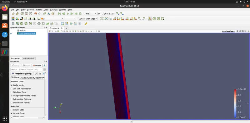
Para view is used for post processing this can be viewed using parafoam command in Terminal.
OUTPUT:
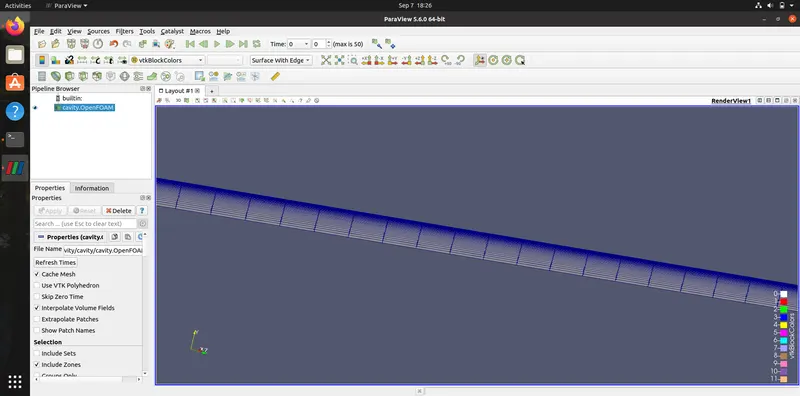
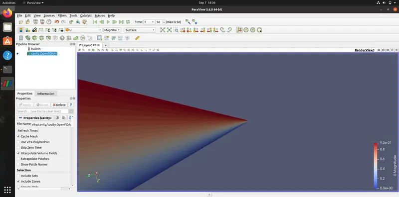
Velocity Profile:
Pressure:
Shear Stress:
RESULTS:
1. The error gradually increases with an increase in wedge length whereas it decreases as well with finer mesh o the profile.
2. Haigen-Poiseuille equation satisfies the numerical analysis of the equation.