Week 11 - Simulation of Flow through a pipe in OpenFoam
this reportis about a simulation of an axi-symmetric flow by applying the wedge boundary condition. The flow is laminar and flows through a constant cross-section pipe at an inlet Reynold's number of 2100.
we assume for a our simulation :
D=0.01m
angle theta=4°
so here is the main program which give us the blockMeshfile automatically:
clear all
close all
clc

D=input('give a value for the diameter:');
L=input('give a value for length:');
alpha=input('give a value for the angle thetha for your element volume:');
rho=input('density:');
filename='blockMeshDict';
u=input('give a value for dynamic viscosity:');
Pi=100;
Po=0;
Re=2100;
n=93; %number of lines inside the text file
vertices_start=20; %the start line of vertices "coordinates of first vertice" it must not have an empty line between the vertices in the blockMesh text
[r,v,Vmax,P_D,Lh]=blockMesh_generation(alpha,L,D,filename,u,rho,Re,vertices_start,n);

%plot(r,v)
and the subprogram which will be called by this program is:
function [r,v,Vmax,P_D,Lh]=blockMesh_generation(alpha,L,D,filename,u,rho,Re,vertices_start,n)


Vavg=(Re*u)/(rho*D)

Vmax=Vavg*2  %Maximum velocity

P_D=(32*u*Vavg)/D^2 %pressure drop
R=D/2;
t=L/Vmax


r=linspace(0,R,100);
v=2*Vavg*(1-r.^2/R^2);  %analytical velocity profile

Lh=0.05*Re*D;


f1=fopen(filename,'r'); %read the file

for i=1:n           %to point into the reference of the next line
    line{i}=fgetl(f1);% copy the next line

end
fclose(f1);

% R=1;
% L=10;
% alpha=5;
% %vertices
 x=R*sind(alpha/2);
 y=R*cosd(alpha/2);
 z1=0;
 z2=L;

n_line=vertices_start;

line{n_line}='';  %n_line: line number n
str='    (0 0 0)';
ln=length(str);
line{n_line}(1:ln)=str;
n_line=n_line+1;

str=sprintf('     (%.10f %.10f %.10f)',z1,y,x);
ln=length(str);
line{n_line}='';
line{n_line}(1:ln)=str;
n_line=n_line+1;

str=sprintf('     (%.10f %.10f %.10f)',z1,y,-x);
ln=length(str);
line{n_line}='';
line{n_line}(1:ln)=str;
n_line=n_line+1;

str=sprintf('     (%.10f %.10f %.10f)',z2,0,0);
ln=length(str);
line{n_line}='';
line{n_line}(1:ln)=str;
n_line=n_line+1;

str=sprintf('     (%.10f %.10f %.10f)',z2,y,x);
ln=length(str);
line{n_line}='';
line{n_line}(1:ln)=str;
n_line=n_line+1;

str=sprintf('     (%.10f %.10f %.10f)',z2,y,-x);
ln=length(str);
line{n_line}='';
line{n_line}(1:ln)=str;


f1=fopen('blockMeshDict2','w');
for j=1:n
    fprintf(f1,'%s',line{j}(1:end));
    fprintf(f1,'\n');
end
fclose(f1);
which gives at the end of the day:
/*--------------------------------*- C++ -*----------------------------------*\
  =========                 |
  \\      /  F ield         | OpenFOAM: The Open Source CFD Toolbox
   \\    /   O peration     | Website:  https://openfoam.org
    \\  /    A nd           | Version:  8
     \\/     M anipulation  |
\*---------------------------------------------------------------------------*/
FoamFile
{
     version 	 2.0;
      format 	 ascii;
       class 	 dictionary;
      object 	 blockMeshDict;
)

convertToMeters 1;

vertices
(
    (0 0 0)
     (0.0000000000 0.0049969541 0.0001744975)
     (0.0000000000 0.0049969541 -0.0001744975)
     (2.5000000000 0.0000000000 0.0000000000)
     (2.5000000000 0.0049969541 0.0001744975)
     (2.5000000000 0.0049969541 -0.0001744975)
);

blocks
(
	 hex (0 3 5 2 0 3 4 1) (200 20 1) SimpleGrading (1 0.1 1)

);

edges
(
	 arc 1 2 (0 7.500000e-03 0)
	 arc 4 5 (2.500000e+00 7.500000e-03 0)
);

boundary
(
	 inlet
	 {
		 type patch;
		 faces
		 (
			 (0 1 2 0)
		);
	 }
	 outlet
	 {
		 type patch;
		 faces
		(
			 (3 5 4 3)
		);
	 }
	 top
	 {
		 type wall;
		 faces
		(
			 (1 4 5 2)
		);
	 }
	 front
	 {
		 type wedge;
	 faces
		(
			 (0 3 4 1)
		);
	 }
	 back
	 {
		 type wedge;
	 faces
		(
			 (0 2 5 3)
		);
	 }
	 axis
	 {
		 type empty;
	 faces
		(
			 (0 3 3 0)
		);
	 }
);
mergePatchPairs
(
);
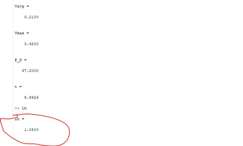
1. Validate Hydro-dynamic length with the numerical result:
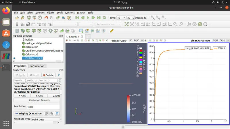
as you see in the ghraphe the velocity along x axis start becoming constant from x=1.055 which match with the analytical results:
2.Validate the fully developed flow velocity profile with its analytical profile:
clear all
close all
clc
%inputs
R=0.01/2;
Vavg=0.21;


f1=fopen('weeek11.txt','r'); %read the file
line{1}=fgetl(f1);
line{2}=fgetl(f1);%copy the first line into a dictionarry called line


for i=2:1002


    num_line=str2num(line{i});
    nm_line1=num_line(1);
    nm_line2(i)=num_line(2);
    v(i)=2*Vavg*(1-nm_line1^2/R^2);
    i=i+1; %to point into the reference of the next line
    line{i}=fgetl(f1);% copy the next line


end
line=line(1:end-1);%delete the last element cause it includes[-1](the stop condition for the while loop)
fclose(f1)

%analytical velocity along y axis
plot(v)
hold on
%numerical velocity
plot(nm_line2)
legend('analytical','numerical')
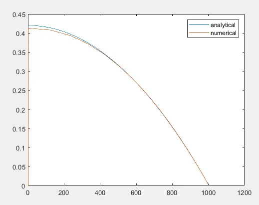
the analytical and the numeical results from openfoam match at the end
3.Validation maximum velocity and pressured drop for fully developed flow:
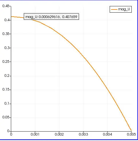
maximum velocity:
pressure_drop:
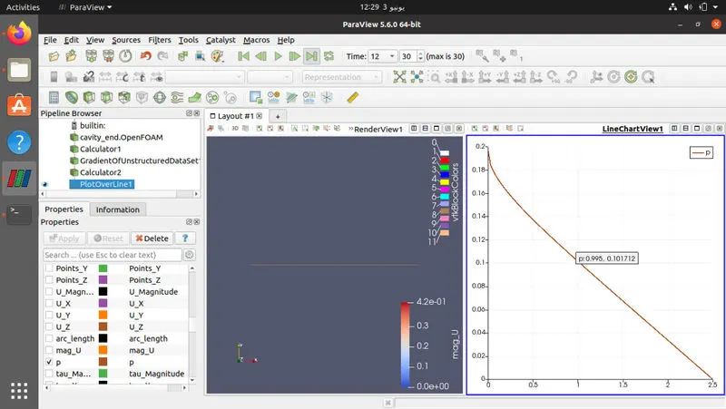
maximum velocity and pressure drop match witha analytical results calculated on matlab:
%part of the subprogram
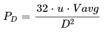
P_D=(32*u*Vavg)/D^2 %pressure drop
R=D/2;
t=L/Vmax


r=linspace(0,R,100);
v=2*Vavg*(1-r.^2/R^2);  %analytical velocity profile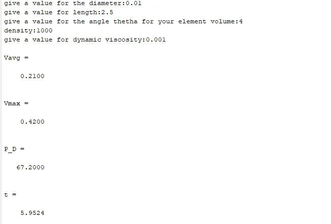
4.Post-process for Shear stress and validation of wall shear stress for fully developed flow
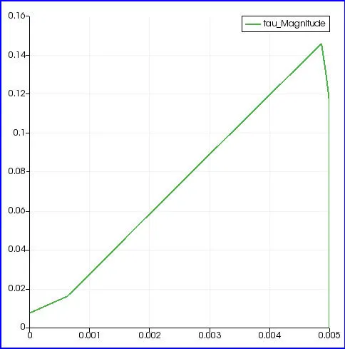
validate our results with the Hagen- Poiseuille's equations for the fully developed flow:
the Hagen- Poiseuille's equations:
analytica results using matlab:
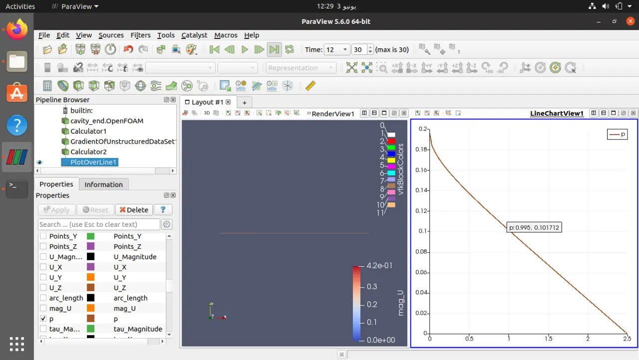
using D=0.01 and D=0.02 , which means D and 2D .And verify with the numerical reusults
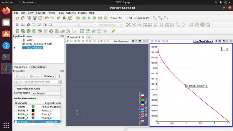
give a value for the diameter:0.02
give a value for length:2.5
give a value for the angle thetha for your element volume:4
density:1000
give a value for dynamic viscosity:0.001

Vavg =

    0.1050


Vmax =

    0.2100


P_D =

    8.4000


t =

   11.9048

>> 0.013/1.5

ans =

    0.0087

>> ans*rho

ans =

    8.6667

>> 
give a value for the diameter:0.01
give a value for length:2.5
give a value for the angle thetha for your element volume:4
density:1000
give a value for dynamic viscosity:0.001

Vavg =

    0.2100


Vmax =

    0.4200


P_D =

   67.2000


t =

    5.9524

>>
So the Hagen- Poiseuille's equation is verified as we see when we double the value of diametre ,pressure drop by a factor of 2^3.
Conclusion:
the analytical results and the numericals one have a high level of match ,so we can depend on openfoam to do others simulation sand making sure that it gives good results.