Week 5 - Mid term project - Solving the steady and unsteady 2D heat conduction problem
In this work we will try to reach the profile of the temperature in a 2D plan ,in two cases :steady state and unsteady state .We will work with implicit and explicit scheme for the unsteady state ,and implicit state for steady state .
- unsteady equation with implicit scheme
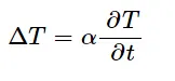 we converte this equation into algebric form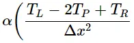
 using the central difference for derivatives.
we will use three methode starting with jacobi methode ,which insiste to compute the actuale value with the last iteration values with this expression :

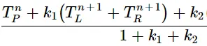
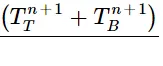 with
with 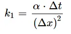 and
and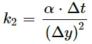 .
.
then the Guauss methode which use the current obtained values of TL and TB.
and finally the Sor methode obtained from taylor series :
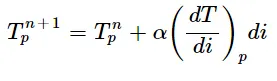 , with some rearangment through replacing dT/di by jacobi or Gauss
 we get:

here is the program which output the temperature profile in 2D plan after some interval of time t:
%iterative methode for unsteady conduction equation in implicit scheme


clear all
close all
clc

%number of nodes  along x axis
nx=50;
ny=50;
T=300*ones(nx,ny);        %intializing inner nodes to 300K
T(2:end-1,1)=(400/300)*T(2:end-1,1); %right Boundary
T(1,2:end-1)=(900/300)*T(1,2:end-1); %Bottom Boundary
T(2:end-1,end)=(800/300)*T(2:end-1,end); %Left boundary
T(end,2:end-1)=(600/300)*T(end,2:end-1); %Top boundary
%computing the corners boundariens
T(1,1)=(T(1,2)+T(2,1))/2;
T(end,end)=(T(end-1,end)+T(end,end-1))/2;
T(end,1)=(T(end-1,1)+T(end,2))/2;
T(1,end)=(T(2,end)+T(1,end-1))/2;
%step time
dt=1;
% t=linspace(0,100*dt,dt);

%space interval
x=linspace(0,1,nx);
dx=1/(nx-1);
y=linspace(0,1,ny);
dy=1/(ny-1);
%getting the 2D plan
[xx,yy]=meshgrid(x,y);

%which iterative methode we want to use
txt='which iterative methode you want to use:'
iterative_solver=input(txt)

%creating a copy of T
Told=T;

%absolute error criteria
tol= 1e-4;

%unsteady equation of heat conduction

%inputing constants
a=1.5;
k1=a*dt/dx^2;
k2=a*dt/dy^2;
term1=(1+2*k1+2*k2)^-1;
term2=term1*k1;
term3=term1*k2;

%save the previous Temperature profile
T_prev_dt=T;


%jacobi methode
if iterative_solver==1
    jacobi_iter=0;
    for nt=1:10 %time loop
        error=1;
        while error>tol %convergence loop
            for i=2:nx-1 %space loop
                for j=2:ny-1
                    H=Told(i-1,j)+Told(i+1,j);
                    V=Told(i,j-1)+Told(i,j+1);
                    T(i,j)=(T_prev_dt(i,j)*term1)+(H*term2)+(V*term3);
                end
            end
            error= max(max(abs(Told-T))); %verifying the convergence
            Told=T; %save the temperature profile
            jacobi_iter=jacobi_iter+1;

            %contourf(xx,yy,T);% plotting
%             title_text=sprintf('iteration_number=%d',jacobi_iter);
%             title(title_text); %giving a title which mention the actual iterative


        end
        T_prev_dt=T ;
    end
    %C=contourf(xx,yy,T);
     C=contourf(xx,yy,T);% plotting
     clabel(C,'FontWeight','bold');
     title1=sprintf('jacobi methode for steady heat conduction equantion with %d iterations',jacobi_iter)
     title(title1)
     xlabel 'x axis'
     ylabel 'y axis'
end


if iterative_solver==2
%Guauss methode
Gs_iter=1;
    for nt=1:100
            error=1;
            while error>tol
                for i=2:nx-1
                    for j=2:ny-1
                        H=T(i-1,j)+T(i+1,j); % simple changement in compare to the jacobi methode
                        V=T(i,j-1)+T(i,j+1);% by using the actual available temperatue values in its (x,y) position
                        T(i,j)=(T_prev_dt(i,j)*term1)+(H*term2)+(V*term3);
                    end
                end
                error= max(max(abs(Told-T)));
                Told=T;
                Gs_iter=Gs_iter+1;


            end
    T_prev_dt=T ;
    end


     C=contourf(xx,yy,T);% plotting
     clabel(C,'FontWeight','bold');
     title1=sprintf('Gauss methode for steady heat conduction equantion with %d iterations',Gs_iter)
     title(title1)
     xlabel 'x axis'
     ylabel 'y axis'
end

if iterative_solver==3
    %Rso methode
       Rso_iter=0;
       a=1.6; %relaxation factor
        for nt=1:100
            error=1;
            while error>tol
                for i=2:nx-1
                    for j=2:ny-1
                        H=T(i-1,j)+T(i+1,j);
                        V=T(i,j-1)+T(i,j+1);
                        T(i,j)=Told(i,j)*(1-a)+a*((T_prev_dt(i,j)*term1)+(H*term2)+(V*term3)); % Rso methode using guauss expression

                    end
                end
                error= max(max(abs(Told-T)));
                Told=T;
                Rso_iter=Rso_iter+1;


            end
        T_prev_dt=T ;
    end


     %C=contourf(xx,yy,T);
     C=contourf(xx,yy,T);% plotting
     clabel(C,'FontWeight','bold');
     title1=sprintf('RSO methode for steady heat conduction equantion with %d iterations',Rso_iter)
     title(title1)
     xlabel 'x axis'
     ylabel 'y axis'
end
Plots:
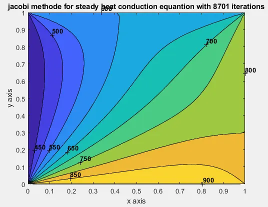
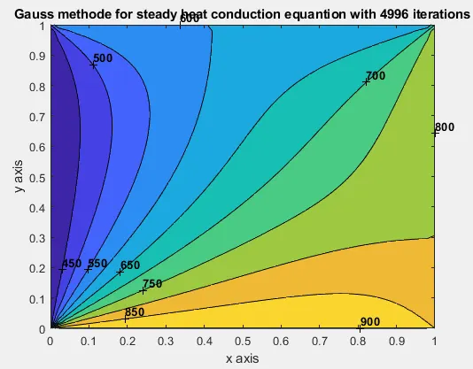
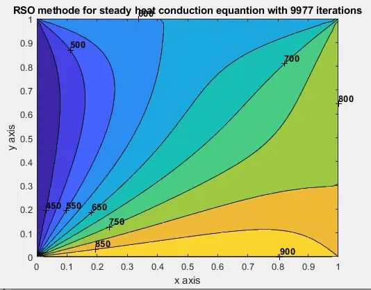 for a factor relaxation a=0.6.
we can notice that all the plots are the same except each of them require a specific number of iterations, each one require different number pf iterations.
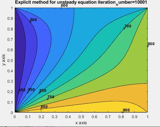
These graphes include the meaning of how temperature will be distribute a 2D plan like a plate with a thickness tending to 0.
2-Explicit methode for unsteady equation :
 =
=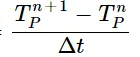
which lead to:


And here is the program that compute this temperature profile at each time step.
%EXPLICIT METHOD FOR unsteady equation

clear all

clc
%number of nodes  along x axis
nx=100;
ny=100;
T=ones(ny,nx);
T=T*300;
%Assigning BC
T(2:end-1,1)=(400/300)*T(2:end-1,1); %right Boundary
T(1,2:end-1)=(900/300)*T(1,2:end-1); %Bottom Boundary
T(2:end-1,end)=(800/300)*T(2:end-1,end); %Left boundary
T(end,2:end-1)=(600/300)*T(end,2:end-1); %Top boundary
T(1,1)=(T(1,2)+T(2,1))/2;
T(end,end)=(T(end-1,end)+T(end,end-1))/2;
T(end,1)=(T(end-1,1)+T(end,2))/2;
T(1,end)=(T(2,end)+T(1,end-1))/2;
dt=0.00001;
% t=linspace(0,1400*dt,dt);


x=linspace(0,1,nx);
dx=1/(nx-1);
y=linspace(0,1,ny);
dy=1/(ny-1);

[xx,yy]=meshgrid(x,y)

%creating a copy of T
Told=T;
T_prev_dt=T;
a=2;
k1=a*dt/dx^2;
k2=a*dt/dy^2;
term1=(1-2*k1-2*k2);
term2=k1;
term3=k2;


iter=1;
for nt=1:10000
            for i=2:nx-1
                for j=2:ny-1
                    H=Told(i-1,j)+Told(i+1,j);
                    V=Told(i,j-1)+Told(i,j+1);
                    T(i,j)=(T_prev_dt(i,j)*term1)+(H*term2)+(V*term3);
                end
            end

            Told=T;
            iter=iter+1;
            T_prev_dt=T;
end

 C=contourf(xx,yy,T);
 clabel(C,'FontWeight','bold');
 title_text=sprintf('Explicit method for unsteady equation iteration_number=%d',iter);
 title(title_text);
 xlabel 'x axis'
 ylabel 'y axis'
Ploting result:
3-unsteady equation with implicit scheme
 we converte this equation into algebric form
 using the central difference for derivatives.
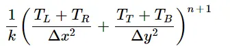
we will use three methode starting with jacobi methode ,which insiste to compute the actuale value with the last iteration values with this expression :
 with .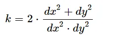
then the Guauss methode which use the current obtained values of TL and TB.
and finally the Sor methode obtained from taylor series :
, with some rearangment through replacing dT/di by jacobi or Gauss we get:
here is the program which output the temperature profile in 2D plan after some interval of time t
%2D steady conduction equt with implicit scheme

clear all
close all
clc
%number of nodes  along x axis
nx=100;
ny=100;
T=ones(ny,nx);
T=T*300;
%Assigning BC
T(2:end-1,1)=(400/300)*T(2:end-1,1); %right Boundary
T(1,2:end-1)=(900/300)*T(1,2:end-1); %Bottom Boundary
T(2:end-1,end)=(800/300)*T(2:end-1,end); %Left boundary
T(end,2:end-1)=(600/300)*T(end,2:end-1); %Top boundary
%computing the corners boundaries
T(1,1)=(T(1,2)+T(2,1))/2;
T(end,end)=(T(end-1,end)+T(end,end-1))/2;
T(end,1)=(T(end-1,1)+T(end,2))/2;
T(1,end)=(T(2,end)+T(1,end-1))/2;


%gerating space
x=linspace(0,1,nx);
dx=1/(nx-1);
y=linspace(0,1,ny);
dy=1/(ny-1);
%getting the 2D plan
[xx,yy]=meshgrid(x,y);

%which iterative methode we want to use
txt='which iterative methode you want to use:';
iterative_solver=input(txt);

%creating a copy of T
Told=T;
%absolute error criteria
tol= 1e-04;
error=1;

%solving steady equation of heat conduction

%constant for simplification
k=2*(dx^2+dy^2)/(dx^2*dy^2);


%jacobi methode
if iterative_solver==1
    jacobi_iter=0;
    while error>tol

                for i=2:nx-1
                    for j=2:ny-1
                        term1=(Told(i-1,j)+Told(i+1,j))/dx^2;
                        term2=(Told(i,j-1)+Told(i,j+1))/dy^2;
                        T(i,j)=(1/k)*(term1+term2);
                    end
                end
                error= max(max(abs(Told-T)));
                Told=T;
                jacobi_iter=jacobi_iter+1;
                %contourf(xx,yy,T)
                %title_text=sprintf('iteration number=%d',jacobi_iter)
                %title(title_text)
                %pause(0.3)

    end
     C=contourf(xx,yy,T);
     clabel(C,'FontWeight','bold');
     title_text=sprintf('Implicit jacobi method for steady equation iteration_number=%d',jacobi_iter);
     title(title_text);
     xlabel 'x axis'
     ylabel 'y axis'
end

if iterative_solver==2
%Guauss methode
    Gs_iter=1;
        for nt=1:100
                error=1;
                while error>tol
                    for i=2:nx-1
                        for j=2:ny-1
                            term1=(Told(i-1,j)+Told(i+1,j))/dx^2;
                            term2=(Told(i,j-1)+Told(i,j+1))/dy^2;
                            T(i,j)=(1/k)*(term1+term2);
                        end
                    end
                    error= max(max(abs(Told-T)));
                    Told=T;
                    Gs_iter=Gs_iter+1;
    %                 C=contourf(xx,yy,T);
    %                 title_text=sprintf('iteration_number=%d',Gs_iter);
    %                 title(title_text);
    %                 pause(0.2)


            end
    end

     C=contourf(xx,yy,T);
     clabel(C,'FontWeight','bold');
     title_text=sprintf('Implicit Gauss method for steady equation iteration_number=%d',Gs_iter);
     title(title_text);
     xlabel 'x axis'
     ylabel 'y axis'
end

if iterative_solver==3
    %Rso methode
       Rso_iter=0;
       a=0.6; %relaxation factor
        for nt=1:100
            error=1;
            while error>tol
                for i=2:nx-1
                    for j=2:ny-1
                        term1=(Told(i-1,j)+Told(i+1,j))/dx^2;
                        term2=(Told(i,j-1)+Told(i,j+1))/dy^2;
                        T(i,j)=Told(i,j)*(1-a)+a*((1/k)*(term1+term2)); % Rso methode using guauss expression

                    end
                end
                error= max(max(abs(Told-T)));
                Told=T;
                Rso_iter=Rso_iter+1;
%                 C=contourf(xx,yy,T);
%                 title_text=sprintf('iteration_number=%d',Rso_iter);
%                 title(title_text);
%                 pause(0.2)


            end
    end

     C=contourf(xx,yy,T);
     clabel(C,'FontWeight','bold');
     title_text=sprintf('Implicit RSO method for steady equation iteration_number=%d',Rso_iter);
     title(title_text);
     xlabel 'x axis'
     ylabel 'y axis'
 end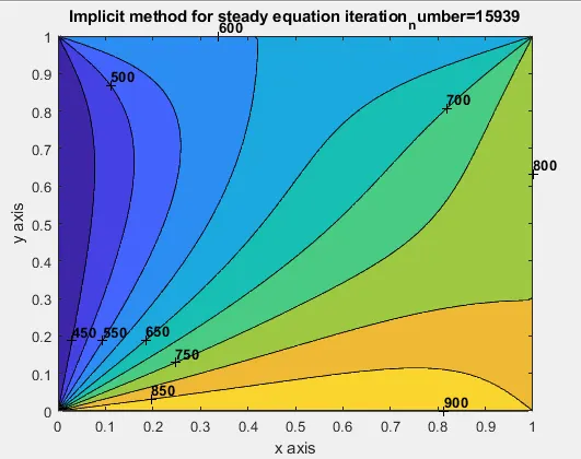
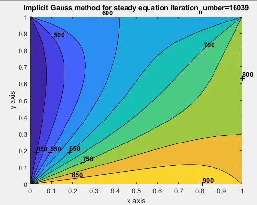
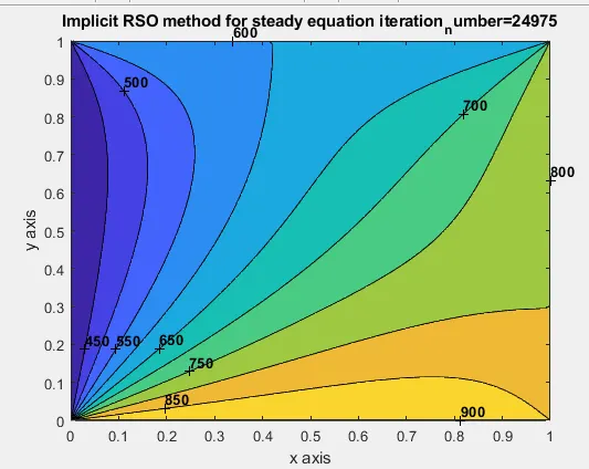
The number of iteration is very large but at the end it gives the same results.