Week 8 - Simulation of a backward facing step in OpenFOAM

In this report i am going to describe my PreProcessing and PostProcessing of the simulation of an incompressible laminar fluid flow in OpenFoam. Indeed, the PreProcessing involve the generation of the mesh in some way to get the desirable shape in which the fluid flow is going to be simulated. In the other hand ,when i go for the PostProcessing i will analyse velocity data in a specific regio ,and try to figure out how the grading factor influence results.

pre processing:

i named my shape nodes as follow:

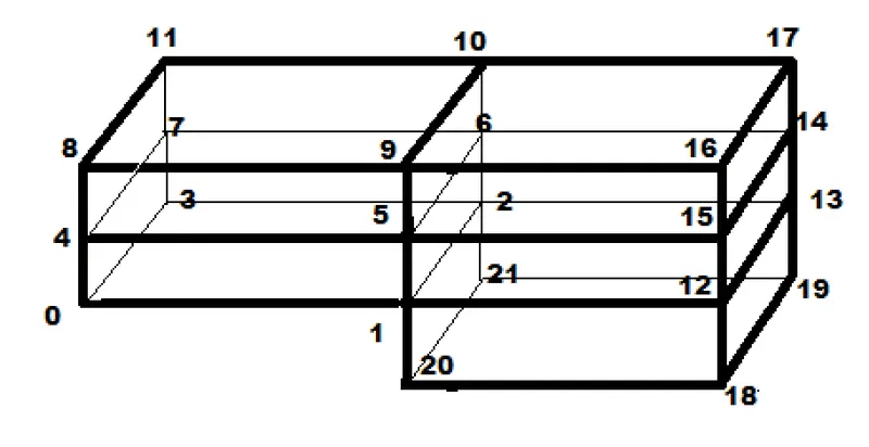
which i should define in the blockMesh file in section vertices:

convertToMeters 0.1;

vertices
(
    (0 0 0)
    (1 0 0)
    (1 1 0)
    (0 1 0)
    (0 0 0.1)
    (1 0 0.1)
    (1 1 0.1)
    (0 1 0.1)
    //block 2
    (0 0 0.2)
    (1 0 0.2)
    (1 1 0.2)
    (0 1 0.2)
    
    (2 0 0)
    (2 1 0)
    (2 1 0.1)    
    (2 0 0.1)
    
    (2 0 0.2)    
    (2 1 0.2)
 
    (2 0 -0.2)    
    (2 1 -0.2)
    (1 0 -0.2)
    (1 1 -0.2)

then we need to define the nature of every walls, where in this case we have only one moving wall which is (0 4 7 3) and (4 8 11 7):

boundary
(
    movingWall
    {
        type wall;
        faces
        (
        
        (0 4 7 3)
        (4 8 11 7)      
   
        );
       
    }
    fixedWalls
    {
        type wall;
        faces
        (
            
      
            
            (3 7 6 2) 
            (7 11 10 6)
            (2 6 14 13)
            
            (12 13 14 15)
            (15 14 17 16)
            
            (12 18 19 13)
            (1 2 21 20)
            
            (10 17 14 6)
            (2 13 19 21)
            
        (1 5 4 0)
        (5 9 8 4)
        (1 12 15 5)
        (5 15 16 9)
        (20 18 12 1)
            
            
            
        );
    }
    frontAndBack
    {
        type empty;
        faces
        (
        
        
        (0 3 2 1)
        (8 9 10 11)
        
        (9 10 17 16)
        (20 21 19 18)
        
            
            
        );
    }
);

after that we must define every blocks as we see in the first image:

locks
(
    hex (0 1 2 3 4 5 6 7) (50 20 1) simpleGrading (1 1 1)
    hex (4 5 6 7 8 9 10 11) (50 20 1) simpleGrading (1 1 1)
    hex (1 12 13 2 5 15 14 6) (50 20 1) simpleGrading (1 1 1)
    hex (5 15 14 6 9 16 17 10) (50 20 1) simpleGrading (1 1 1)
    hex ( 20 18 19 21 1 12 13 2) (50 20 1) simpleGrading (1 1 1)
);

(50 20 1) :means that we have 50 grid along the x axis and 20 grid along the y axis and 1 grid in the z axix for this block.

simpleGrading(0.1 1 1): 0.1 refers to the size of the end cell compared to the first one along the x axis ,and the cells between these last two keep decreasing or incecreasing ,if we whave (10 1 1) as an example ,along the x axis. The same thing in y axis and z axis we just need to act one the second input and the third input respectively:( 1 0.1 1) and (1 1 0.1).

Now we should choose the reference case file that allow us to run a simulation of an incompressible-laminar-viscous flow .

When we search we found that the file named IcoFoam inside of the file Incompressible in tutorials files gives us that kind of simulation.

So now we are ready to launch the simulation, but before that we need to apply the boundary condition by applying 0 in x and z component of velocity and 1 in the y component ,for that we proced as follow:

we go to a file named 0 where we find a script named U which contains the initial profile of velocity by taping: ~/OpenFOAM/ahmedmtbrk-8/run/cavity_sim/0$ gedit U, so we get :

/*--------------------------------*- C++ -*----------------------------------*\
  =========                 |
  \\      /  F ield         | OpenFOAM: The Open Source CFD Toolbox
   \\    /   O peration     | Website:  https://openfoam.org
    \\  /    A nd           | Version:  8
     \\/     M anipulation  |
\*---------------------------------------------------------------------------*/
FoamFile
{
    version     2.0;
    format      ascii;
    class       volVectorField;
    object      U;
}
// * * * * * * * * * * * * * * * * * * * * * * * * * * * * * * * * * * * * * //

dimensions      [0 1 -1 0 0 0 0];

internalField   uniform (0 0 0);

boundaryField
{
    movingWall
    {
        type            fixedValue;
        value           uniform (0 1 0);
    }

    fixedWalls
    {
        type            noSlip;
    }

    frontAndBack
    {
        type            empty;
    }
}

// ************************************************************************* //

we go to the "moving wall" object

        value           uniform (1 0 0);

this line means that only the x componenet of velocity which not null and equal to 1

so we change to :

        value           uniform (0 1 0);

and we save the file.

we did copy the file named cavity from tutorials/incompressible/icoFoam adress file ,to the run file .

Now we cans launch the simulation by applying the blockmesh using the command "blockMesh" inside the cacity file to run in the terminal:

then we run the simulation by taping the name of the file fromwhere we extract our "cavity" file which is "icoFoam".

and we go to the paview to show aour results by taping in the terminal "paraFoam":

PostProcessing :

we have to cases to studie:

Case 1: Simulating the flow without using any grading factor .

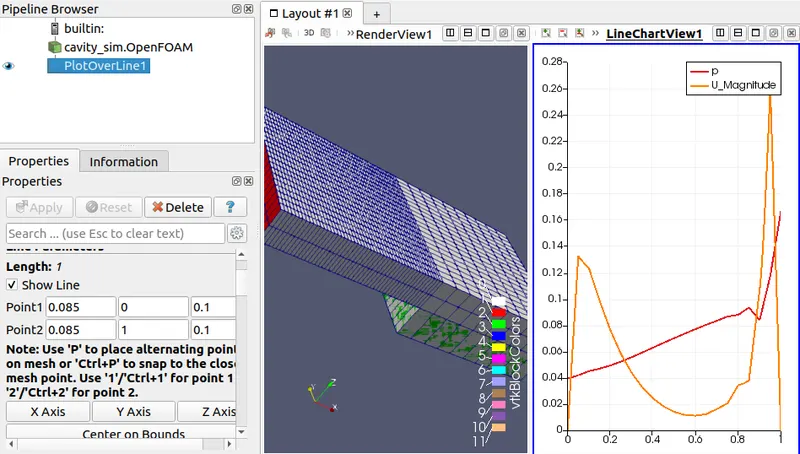
x=50 grids ; y=20 grids ; z=1 grid GF=1. for the two first blocks.

with this changement inside the blockMesh file

blocks
(
    hex (0 1 2 3 4 5 6 7) (50 20 1) simpleGrading (1 1 1)
    hex (4 5 6 7 8 9 10 11) (50 20 1) simpleGrading (1 1 1)
    hex (1 12 13 2 5 15 14 6) (10 20 1) simpleGrading (1 1 1)
    hex (5 15 14 6 9 16 17 10) (10 20 1) simpleGrading (1 1 1)
    hex ( 20 18 19 21 1 12 13 2) (10 20 1) simpleGrading (1 1 1)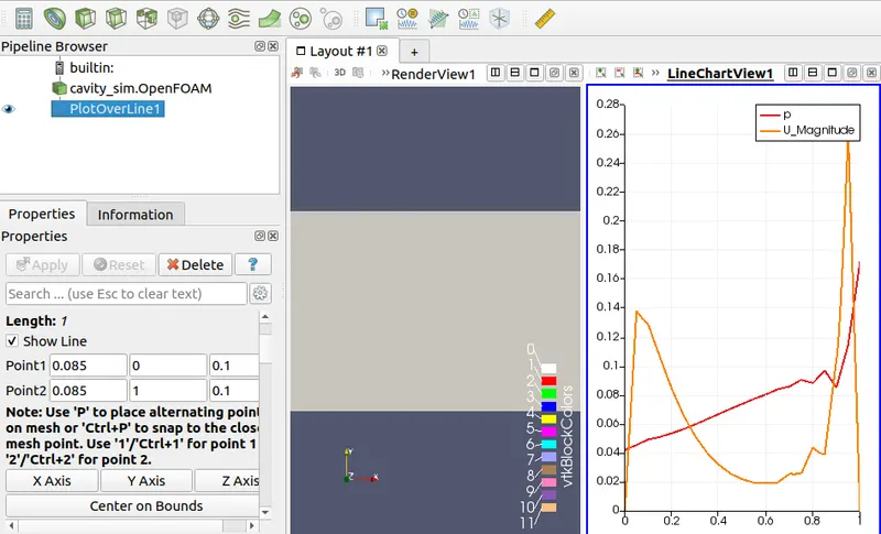

x=100 grids ; y=20 grids ; z=1 grid GF=1.

blocks
(
    hex (0 1 2 3 4 5 6 7) (100 20 1) simpleGrading (1 1 1)
    hex (4 5 6 7 8 9 10 11) (100 20 1) simpleGrading (1 1 1)
    hex (1 12 13 2 5 15 14 6) (10 20 1) simpleGrading (1 1 1)
    hex (5 15 14 6 9 16 17 10) (10 20 1) simpleGrading (1 1 1)
    hex ( 20 18 19 21 1 12 13 2) (10 20 1) simpleGrading (1 1 1)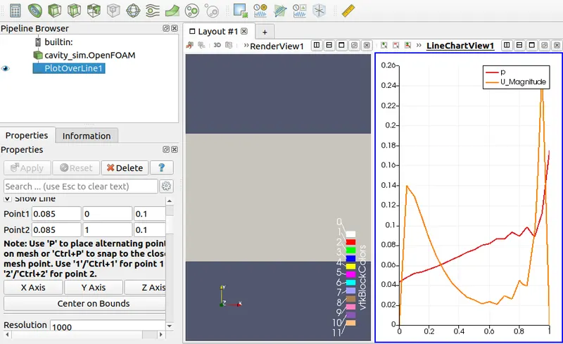

x=200 grids ; y=20 grids ; z=1 grid GF=1.

blocks
(
    hex (0 1 2 3 4 5 6 7) (200 20 1) simpleGrading (1 1 1)
    hex (4 5 6 7 8 9 10 11) (200 20 1) simpleGrading (1 1 1)
    hex (1 12 13 2 5 15 14 6) (10 20 1) simpleGrading (1 1 1)
    hex (5 15 14 6 9 16 17 10) (10 20 1) simpleGrading (1 1 1)
    hex ( 20 18 19 21 1 12 13 2) (10 20 1) simpleGrading (1 1 1)

*: we get inside this script as follow:

And by making this little changement inside the blockMesh file we can move to the second case:

blocks
(
    hex (0 1 2 3 4 5 6 7) (50 20 1) simpleGrading (20 1 1)
    hex (4 5 6 7 8 9 10 11) (50 20 1) simpleGrading (20 1 1)
    hex (1 12 13 2 5 15 14 6) (10 20 1) simpleGrading (1 1 1)
    hex (5 15 14 6 9 16 17 10) (10 20 1) simpleGrading (1 1 1)
    hex ( 20 18 19 21 1 12 13 2) (10 20 1) simpleGrading (1 1 1)

we get:

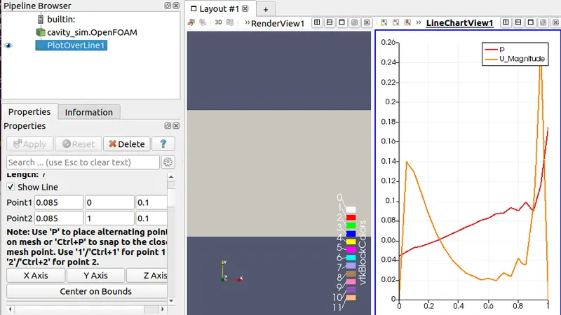
x=50 grids ; y=20 grids ; z=1 grid (GF=20. to get stressed cells near to the moving wall)

x=100 grids ; y=20 grids ; z=1 grid GF=20.

comment:

to extract data with precision near to the walls ,we stressed the cells only in that position so we economise meory and perform the time for running. And we get the same results.

conclusion:

A large number of cells gives us more precision ,but we will have more computer memories occuped through the simulation. So if we used the simplegrading command we will stress the cells in the zone we desire to pick from it our useful data,, by keeping the same number of cells ,so we can gain in term of time simulation and also uncarring about our computer properties.