Week 7 - Simulation of a 1D Super-sonic nozzle flow simulation using Macormack Method

In this work we will deal with deals with the quasi-one-dimensional flow through a convergent-divergent nozzle, we will choose a specific CFD technique ,and the solution will be set up and the procedure will be explained step by step.

We consider the steady, isentropic flow through a convergent-divergent nozzle. The flow at the inlet to the nozzle comes from a reservoir where the pressure and temperature are denoted by p0 , and To, respectively. The cross-sectional area of the reservoir is large ( theoretically, A --+ oo ), and hence thevelocity is very small ( V --+ O)

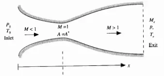
Simulating the flow through the nozzle by deriving the non-conservative equation and conservative form:

Discretisation methode used in this work is named The Macormac method which consist on:

Time marching solution, where we start with an initial conditions and we use it to calculate flow quantities in the next step.

Let F a variable.  We calculate from the governing equations using the forward differencing for space terms then we update  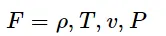using the taylor series as follow ,then we calculate the corrector step from the governing equation .Then we finish by calculating .

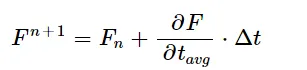predictor step usnig the forward differencing for space terms:

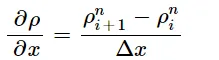
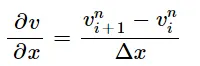
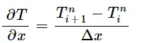
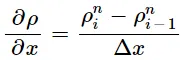
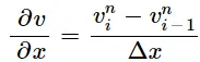
corrector step using the backward differncing for space terms

(partialv)/(partialx)=(v_i^n-v_(i-1)^n)/(Deltax)

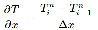
Time derivative expressions:

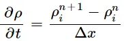
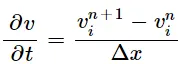
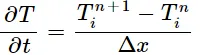
1-non-conservative form

governing equation using The non-conservative equations to solve:

Equation of continuity:

momentum equation:

energy equation:

 ; .

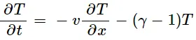
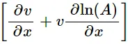these equations are hyperbolic equation.

Here is the sub program code to solve the non-conservative equation:

function [rho,t,v,a,Mfr_steps]=non_conservative1(n,nt)

% inputs  
x=linspace(0,3,n); 
gamma=1.4;
dx=x(2)-x(1);
c=0.5; %assumed CFL number
middle=(n+1)/2;

%Initial profiles
a=1+2.2*(x-1.5).^2;
rho = 1-0.3146*x;
t = 1-0.2314*x;
v =(0.1+1.09*x).*t.^0.5;


dt=min(c*dx./(t.^0.5+v));

for k=1:nt

    rhold=rho;
    vold=v;
    told=t;
    %part one
    %predictor step 
    for j=2:n-1
        dvdx=(v(j+1)-v(j))/dx;
        dlogdx=(log(a(j+1))-log(a(j)))/dx;
        drhodx=(rho(j+1)-rho(j))/dx;
        dtdx=(t(j+1)-t(j))/dx;

        %continuity
        drhodt_p(j)=-rho(j)*dvdx-rho(j)*v(j)*dlogdx-v(j)*drhodx;
        %momentum
        dvdt_p(j)=-v(j)*dvdx-(1/gamma)*(dtdx+(t(j)/rho(j))*drhodx);
        %energy
        dtdt_p(j)=-v(j)*dtdx-(gamma-1)*t(j)*(dvdx+v(j)*dlogdx);

        rho(j)=rho(j)+drhodt_p(j)*dt;
        v(j)=v(j)+dvdt_p(j)*dt;
        t(j)=t(j)+dtdt_p(j)*dt;
    end
    
    %part 2
    %corrector step
    for j=2:n-1
    dvdx=(v(j)-v(j-1))/dx;
    dlogdx=(log(a(j))-log(a(j-1)))/dx;
    drhodx=(rho(j)-rho(j-1))/dx;
    dtdx=(t(j)-t(j-1))/dx;

    %continuity
    drhodt_c(j)=-rho(j)*dvdx-rho(j)*v(j)*dlogdx-v(j)*drhodx;
    %momentum
    dvdt_c(j)=-v(j)*dvdx-(1/gamma)*(dtdx+(t(j)/rho(j))*drhodx);
    %energy
    dtdt_c(j)=-v(j)*dtdx-(gamma-1)*t(j)*(dvdx+v(j)*dlogdx);


    end
    %part three
        %final solution update
    for i=2:n-1
        drhodt_avg(i)=0.5*(drhodt_p(i)+drhodt_c(i));
        dvdt_avg(i)=0.5*(dvdt_c(i)+dvdt_p(i));
        dtdt_avg(i)=0.5*(dtdt_c(i)+dtdt_p(i));
        rho(i)=rhold(i)+drhodt_avg(i)*dt;
        v(i)=vold(i)+dvdt_avg(i)*dt;
        t(i)=told(i)+dtdt_avg(i)*dt;
    end
    %part four
    %apply boundar conditions
    %outlet boudaries
    rho(n)=2*rho(n-1)-rho(n-2);
    v(n)=2*v(n-1)-v(n-2);
    t(n)=2*t(n-1)-t(n-2);
    %Inlet boundaries
%    rho(1)=2*rho(2)-rho(3);
        v(1)=2*v(2)-v(3);
%    t(1)=2*t(2)-t(3);

        R=8.31;

        iter(k)=k;
        rho_t(k)=rho(15);
        v_t(k)=v(15);
        t_t(k)=t(15);
        
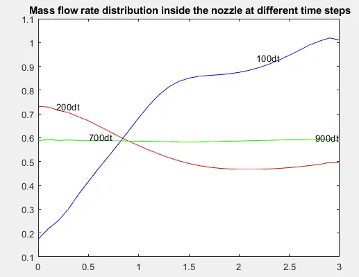
        % Mass flow rate distribution inside the nozzle  
    Mfr_steps=rho.*v.*a;
    
    if k==100
        D1=Mfr_steps;
    end
      
    if k==200
        D2=Mfr_steps;
    end
    
    if k==700
        D3=Mfr_steps;
    end
        
    if k==900
        D4=Mfr_steps;
    end
        
    if k==nt
         figure(4)
         plot(x,D1,'b')
         hold on
         plot(x,D2,'r')
         hold on
         plot(x,D3,'y')
         hold on
         plot(x,D4,'g')
         hold off
         gtext('100dt')
         gtext('200dt')
         gtext('700dt')
         gtext('900dt')
         title(' Mass flow rate distribution inside the nozzle at different time steps')     
    end
        
end         
%Time-wise variation of the primitive variables
figure(5)
subplot(3,1,1)
plot(iter,rho_t)
title('Time-wise variation of the primitive variables')
subplot(3,1,2)
plot(iter,v_t)
subplot(3,1,3)
plot(iter,t_t)
xlabel 'iteration'
    
%Steady-state distribution of primitive variables inside the nozzle
figure(6)
subplot(3,1,1)
plot(x,rho)
title('density inside the nozzle')
subplot(3,1,2)
plot(x,v)
title('velocity inside the nozzle')
subplot(3,1,3)
plot(x,t)
xlabel 'x'
title('temperature inside the nozzle')
end

 Code explanation:

In this code i started by giving the inputs and meshing the space we will working on, then i gived the initial conditions as intitial profiles for each variables Tempertature,density,velocity,area.

Then we we start a time for loop which includs three parts :Using the governing equations and expressions of forward differences we went to calculate the predictor step and update the earlier profiles of primitive variables. The second part was dedicated for backward differences to calculate the predictor step the third part part to give at the end of the day the final results for one time step, we apply boundarie condition to reach the values of each primitive variables in the boundaries by assuming that derivative of each variable at point n and at point n-1 are equale, the same for the side of subsonic flow the derivative at point 1 and point 2 are equal.

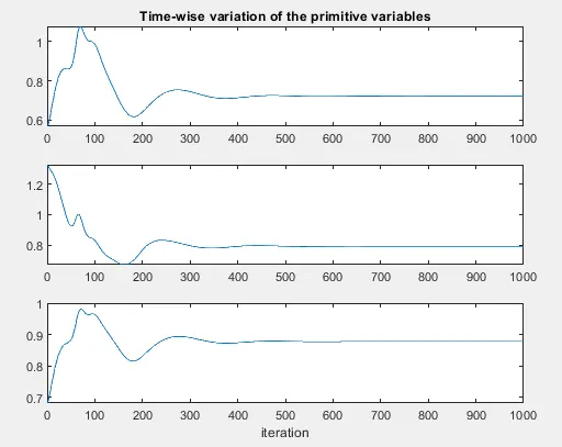
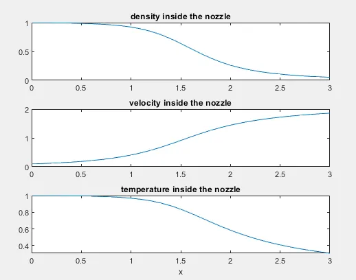
in the end we plot three figures as follow

Steady-state distribution of primitive variables inside the nozzle

 

2-conservative form :

the sub program code to solve the conservative equation:

function [rho,t,v,a,Mfr_steps]=conservative1(n,nt)




%conservative compution 

    gamma=1.4;
    x=linspace(0,3,n);
    dx=x(2)-x(1);
    dt=0.0267;
    middle=(n+1)/2;
    
    %intial density
    rho1=x(1:6).^0;
    rho2=1-0.366*(x(7:16)-0.5);
    rho3= 0.634 - 0.3879*(x(17:end) - 1.5);
    rho=[rho1,rho2,rho3];
    
    %initial temperature
    t1=x(1:6).^0;
    t2=1-0.167*(x(7:16)-0.5);
    t3= 0.833 - 0.3507*(x(17:end) - 1.5);
    t=[t1,t2,t3];
    
    %initial area:
    a=1+2.2*(x-1.5).^2;
    
    %initial velocity
    v=0.59./(rho.*a);
    
    %solution vector
    u1=rho.*a;
    u2=rho.*a.*v;
    u3=rho.*(t./(gamma-1)+0.5*gamma.*v.^2).*a;
    
    %flux terms
    
    
    %source term
%     dlogdx=log(a(2))-log(a);
%     j2=(1/gamma)*(gamma-1)*(u3-0.5*gamma*(u2.^2)./u1)*(1/dx).*(dlogdx);
    
    for i=1:nt
        
        f1=u2;
        f2=(u2.^2)./u1+(1-gamma^-1)*(u3-0.5*gamma*u2.^2./u1);
        f3=gamma*(u2.*u3)./u1-(0.5*gamma)*(gamma-1)*(u2.^3)./(u1.^2);
    
        u1old=u1;
        u2old=u2;
        u3old=u3;
        %predictor step
        for j=2:n-1
            df1dx=(f1(j+1)-f1(j))/dx;
            df2dx=(f2(j+1)-f2(j))/dx;
            df3dx=(f3(j+1)-f3(j))/dx;
            
%             j2(j)=(1/gamma)*(gamma-1)*(u3(j)-0.5*gamma*(u2(j)^2)/u1(j))*(1/dx)*(log(a(j+1))-log(a(j)));
            j2(j)=(1/gamma)*rho(j)*t(j)*((a(j+1))-(a(j)))/dx;
            
            du1dt_p(j)=-df1dx;
            du2dt_p(j)=-df2dx+j2(j);
            du3dt_p(j)=-df3dx;
            
            u1(j)=u1(j)+du1dt_p(j)*dt;
            u2(j)=u2(j)+du2dt_p(j)*dt;
            u3(j)=u3(j)+du3dt_p(j)*dt;
        end
            
        rho=u1./a;
        t=(gamma-1)*(u3./u1-0.5*gamma*v.^2);
        v=u2./u1;
        p=rho.*t;
            
        f1=u2;
        f2=((u2.^2)./u1)+((gamma-1)/gamma)*(u3-((gamma.*u2.^2)./(2*u1)));
        f3=(gamma*u2.*u3./u1)-(0.5*gamma)*(gamma-1)*(u2.^3)./(u1.^2);
            
            
        
        
        %corrector step
        for j=2:n-1
            
            j2(j)=(1/gamma)*rho(j)*t(j)*((a(j)-a(j-1))/dx);
            
            df1dx=(f1(j)-f1(j-1))/dx;
            df2dx=(f2(j)-f2(j-1))/dx;
            df3dx=(f3(j)-f3(j-1))/dx;
            
           
           
            du1dt_c(j)=-df1dx;
            du2dt_c(j)=-df2dx+j2(j);
            du3dt_c(j)=-df3dx;
            
        end
        
%             u1(j)=u1(j)+du1dt*dt;
%             u2(j)=u2(j)+du2dt*dt;
%             u2(j)=u3(j)+du3dt*dt;
        
          du1dt_avg=0.5*(du1dt_c+du1dt_p);
          du2dt_avg=0.5*(du2dt_c+du2dt_p);
          du3dt_avg=0.5*(du3dt_c+du3dt_p);
          
          for m=2:n-1
              u1(m)=u1old(m)+du1dt_avg(m)*dt;
              u2(m)=u2old(m)+du2dt_avg(m)*dt;
              u3(m)=u3old(m)+du3dt_avg(m)*dt;
          end
     %apply boundar conditions
%     outlet boudaries
        u1(n)=2*u1(n-1)-u1(n-2);
        u2(n)=2*u2(n-1)-u2(n-2);
        u3(n)=2*u3(n-1)-u3(n-2);
        
%         f1(n)=u2(n);
%         f2(n)=u2(n)^2/u1(n)+(gamma-1)*(u3(n)-0.5*gamma*u2(n)^2/u1(n))/gamma;
%         f3(n)=gamma*(u2(n)*u3(n))/u1(n)-0.5*gamma*(gamma-1)*u2(n)^3/u1(n)^2;
        
        

%     Inlet boundaries
        u1(1)=rho(1).*a(1);
        u2(1)=2*u2(2)-u2(3);
        u3(1)=u1(1)*(t(1)/(gamma-1)+0.5*gamma*v(1)^2);
        
%         f1(1)=u2(1);
%         f2(1)=u2(1)^2/u1(1)+(gamma-1)*(u3(1)-0.5*gamma*u2(1)^2/u1(1))/gamma;
%         f3(1)=gamma*(u2(1)*u3(1))/u1(1)-0.5*gamma*(gamma-1)*u2(1)^3/u1(1)^2;
        
        rho=u1./a;
        t=(gamma-1)*(u3./u1-0.5*gamma*(u2./u1).^2);
        v=u2./u1;
        
        
        %distribution of primitive variables inside the nozzle
        
        
        %Time-wise variation of the primitive variables
        time=1:1:nt;
        
        rho_middle(i)=rho(middle);
        t_middle(i)=t(middle);
        v_middle(i)=v(middle);
        Mfr_middle(i)=rho(middle)*a(middle)*v(middle);
        

        
      
        % Variation of Mass flow rate distribution inside the nozzle at different time steps 
        %during the time-marching process
        Mfr_steps=rho.*v.*a;
        
        if i==100
            D1=Mfr_steps;
        end
       
        if i==200
            D2=Mfr_steps;
        end
        
        if i==700
            D3=Mfr_steps;
        end
        
        if i==900
            D4=Mfr_steps;
        end
        
        if i==nt
             figure(3)
             plot(x,D1,'b')
             hold on
             plot(x,D2,'r')
             hold on
             plot(x,D3,'y')
             hold on
             plot(x,D4,'g')
             hold off
             gtext('100dt')
             gtext('200dt')
             gtext('700dt')
             gtext('900dt')
             title(' Mass flow rate distribution inside the nozzle at different time steps')
        end
         
         
        %legend('100','200','700','1000')
        
    
    
    end
        figure(1)
        title('distribution of primitive variables inside the nozzle');
        
        subplot(3,1,1)
        plot(x,rho)
        xlabel 'grid points'
        ylabel 'rho/rho_{0}'
        
        subplot(3,1,2)
        plot(x,t)
        xlabel 'grid points'
        ylabel 't/t_{0}'
        
        subplot(3,1,3)
        plot(x,v)
        xlabel 'grid points'
        ylabel 'v/v_{0}'
        
        figure(2)
        subplot(4,1,1)
        plot(rho_middle)
        xlabel 'iteratio n°'
        ylabel 'p/p_{0}'
        
        
        subplot(4,1,2)
        plot(t_middle)
        xlabel 'iteratio n°'
        ylabel 't/t_{0}'
        
        
        subplot(4,1,3)
        plot(v_middle)
        xlabel 'iteratio n°'
        ylabel 'v/v_{0}'
        
        
        subplot(4,1,4)
        plot(Mfr_middle)
        xlabel 'iteratio n°'
        ylabel 'Mfr/Mfr_{0}'
        
                figure(2)
        subplot(4,1,1)
        plot(rho_middle)
        xlabel 'iteratio n°'
        ylabel 'p/p_{0}'
        
        
        subplot(4,1,2)
        plot(t_middle)
        xlabel 'iteratio n°'
        ylabel 't/t_{0}'
        
        
        subplot(4,1,3)
        plot(v_middle)
        xlabel 'iteratio n°'
        ylabel 'v/v_{0}'
        
        
        subplot(4,1,4)
        plot(Mfr_middle)
        xlabel 'iteratio n°'
        ylabel 'Mfr/Mfr_{0}'
       
        
        
        
end

 Code explanation:

the procedure i follow in this code si  the same as the earlier one .However, by referring to ANDERSON CFD book we didn't proceed to calculate directly the primitive variables but we introduced 6 variables which include in their inside all the primitive variables:

 

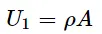
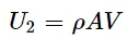
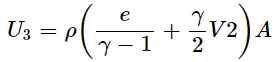
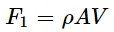
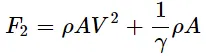
where U is the solution vector and Fthe flux vector and J the source term.

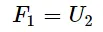
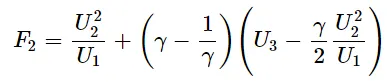
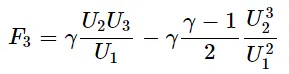
F1, F2, and F3 are couched in terms of the primitive variables, solving the governing equation by constructing F1,F2and F3 at each time step by primitive variables lead to some numerical difficulties until the blow up of the solution.

So we construct them like

with some rearangement we get:

 

we get by the end these plots:

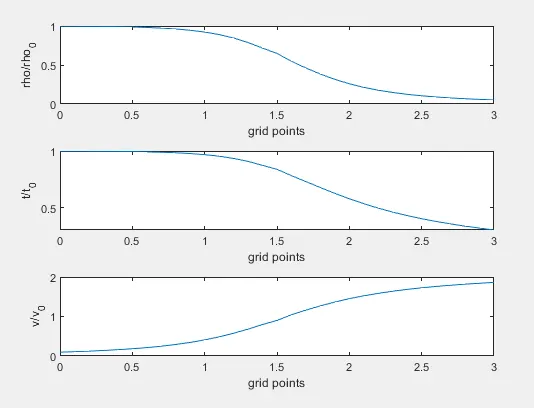
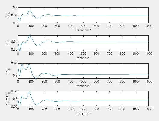
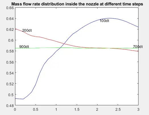
The steady state of both conservative and non-conservative get reached in the same profile at the end

The main progaram that use these two sub program :

clear all 
close all
clc


nt=1000;
n=31;

 [rho_c,t_c,v_c,a_c,Mfr_c]=conservative1(n,nt);
% 
 [rho_n,t_n,v_n,a_n,Mfr_n]=non_conservative1(n,nt);

 
% exact analytical solution of p'A'V' = 0.579 
x=linspace(0,3,n); %meshing
e_a_s=0.579*ones(n); %exact analytical solution
figure(7)
title('Variation of mass flow distributi?n through the nozzle at different times')
hold on
plot(x,Mfr_c)
plot(x,Mfr_n)
plot(x,e_a_s)
xlabel 'x/L'
ylabel 'mass flow rate'
gtext('non-conservative resolver')
gtext('conservative resolver')
gtext('exact analytical solution')

we get this comparaison between the normalized mass flow rate of the conservative and non-conservative form :

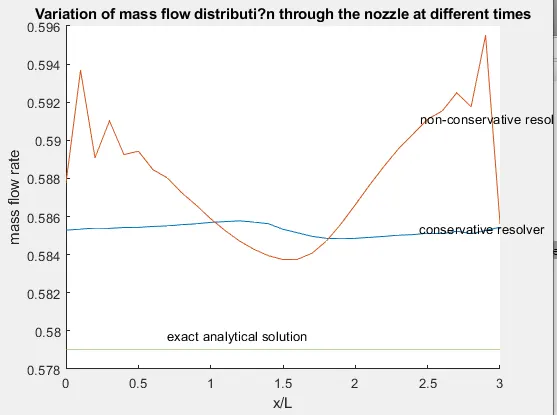
we notice that the conservative form is more stable and close to to the exact analytical solution thus we called the "conservative form"

>> rho_exact=0.634;
>> rho_c(16)-rho_exact

ans =

    0.0147

>> rho_n(16)-rho_exact

ans =

    0.0047

>> t_exact=0.833;
>> t_c(16)-t_exact

ans =

    0.0061

>> t_n(16)-t_exact

ans =

    0.0034

>> 

comparing the results of primitive variables from the conservative and non-conservative form we can conclude that the non conservative form are more accurate than the conservative form.

Conclusion :

1-The conservation form yields a better mass flow distribution. The conservation form simply does a better job of conserving mass.
2-The nonconservation form leads to smaller residuals. The amount by which the residuals decay is often used as an index of "quality" of the numerical algorithm.In this sense, the nonconservation form does a better job.
3. There is no clear superiority of either form in terms of accuracy of the results. The nonconservation form seems to produce slightly more accurate results for the primitive variables, and the conservation form seems to produce slightly more accurate results for the flux variables. The results in either case are certainly satisfactory.