Week 11 - Simulation of Flow through a pipe in OpenFoam
Objective:
- Writing a program in MATLAB that can generate the computational mesh automatically for any wedge angle and grading scheme.
- Show that the velocity profile is fully developed.
- Post-process velocity and shear stress.
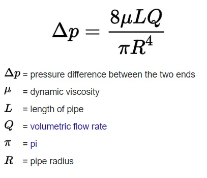
Considering a cylindrical pipe with the working fluid water entering the pipe with the laminar flow. The aim is to simulate the flow through a section of pipe and compare the flow with Hagen Poiseuille’s equation.
In nonideal fluid dynamics, the Hagen–Poiseuille equation, also known as the Hagen–Poiseuille law, Poiseuille law, or Poiseuille equation, is a physical law that gives the pressure drop in an incompressible and Newtonian fluid in laminar flow flowing through a long cylindrical pipe of the constant cross-section. It can be successfully applied to airflow in the lung alveoli, or the flow through a drinking straw or through a hypodermic needle.
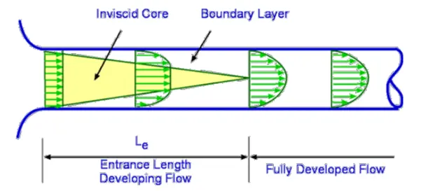
For a pipe with the laminar flow, there are basically two regions. Entrance length developing region where the flow is not fully developed and the laminar flow layers are at equal velocity with respect to each other whereas in the fully developed region the flow is fully developed and follows the Hagen – Poiseuille law.
Assumptions:
- Geometry: Axisymmetric
- Reynolds number Re: 2100 (Laminar Flow)
- Working fluid: water (Density = 998 Kg/m3)
- Fluid Temperature: 25 OC
- Dynamic Viscosity of water = 8.9e-4 Pa-s
- Theta – 4 Degree
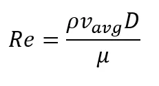
- Calculating the diameter of the pipe (depends on Reynolds number):
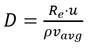
8. For calculating the total length of pipe,
Hydrodynamic Length of the pipe (Lh) = 0.05 * Re * D
Total length of the pipe (L) = Lh + 0.5
Analytical Solution:
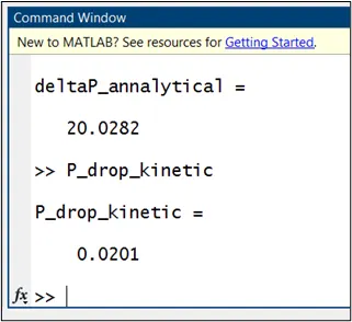
Here for solving the problem numerically we will use the icoFoam solver with the cavity tutorial to make the geometry along with the mesh and make the blockMeshDict file with the help of MATLAB as shown below.
[MATLAB CODE]
clear all
close all
clc

%% Inputs

Re = 2100;                                              % Reynolds No. as mentioned in question
theta = input('Please enter the wedge angle ');         % Angle of Sector of pipe in Degrees
V_avg = input('Please enter the average velocity ');    % Average Velocity
Nu = 1e-6;                                              % Kinematic Viscosity
rho = 998;                                              % Desity of water
V_max = 2*V_avg;                                        % Maximum velocity
mu = 8.9e-4;                                            % Dynamic viscosity of water at 25 Degree celcius
D = (Re*mu)/(rho*V_avg);                                % Diameter of pipe in meters (Calculated according to Reynold's No.)
R = D/2;                                                % Radius of pipe

% Actual Length of pipe
Lh = 0.05*Re*D;                                         % Hydrodynamic length of pipe
L = Lh + 0.5;

%% To calculate the end time of the Simulation

start_time = 0;
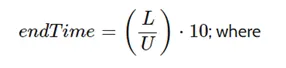
end_time = (L/V_avg);           % Time = Distance/Speed

%% Annalytical Pressure Drop
deltaP_annalytical = ((8*mu*L*V_avg)/R^2);

%% Kinetic Pressure Drop
P_drop_kinetic = deltaP_annalytical/rho;

%% Vertices creation

% Point 0:
x0 = 0;
y0 = 0;
z0 = 0;

% Point 1:
x1 = R*sind(theta/2);
y1 = R*cosd(theta/2);
z1 = 0;

% Point 2:
x2 = -R*sind(theta/2);
y2 =  R*cosd(theta/2);
z2 =  0;

% Point 3:
x3 = 0;
y3 = 0;
z3 = L;

% Point 4:
x4 = R*sind(theta/2);
y4 = R*cosd(theta/2);
z4 = L;

% Point 5:
x5 = -R*sind(theta/2);
y5 =  R*cosd(theta/2);
z5 =  L;


%% Points at Arc

% Arc 1-2
x6 = 0;
y6 = R;
z6 = 0;

% Arc 4-5
x7 = 0;
y7 = R;
z7 = L;

%% No. of cells in local Axis

nx =30;
ny = 1;
nz = 500;

%% Grading Factor

gx = 0.05;
gy = 1;
gz = 1;

%% Creating the BLOCKMESHDICT file

f1 = fopen('blockMeshDict.txt','w');

    fprintf(f1,'/*--------------------------------*- C++ -*----------------------------------*\n');
    fprintf(f1,'  =========                |\n');
    fprintf(f1,'  \\      /  F ield         | OpenFOAM: The Open Source CFD Toolbox\n');
    fprintf(f1,'   \\    /   O peration     | Website:  https://openfoam.org\n');
    fprintf(f1,'    \\  /    A nd           | Version:  8\n');
    fprintf(f1,'     \\/     M anipulation  |\n');
    fprintf(f1,'*---------------------------------------------------------------------------*/\n');
    fprintf(f1,'FoamFile\n');
    fprintf(f1,'{\n');
    fprintf(f1,'    version     2.0;\n');
    fprintf(f1,'    format      ascii;\n');
    fprintf(f1,'    class       dictionary;\n');
    fprintf(f1,'    object      blockMeshDict;\n');
    fprintf(f1,'}\n');
    fprintf(f1,'// * * * * * * * * * * * * * * * * * * * * * * * * * * * * * * * * * * * * * //\n\n');
    fprintf(f1,'convertToMeters 1;\n\n');
    fprintf(f1,'vertices\n');
    fprintf(f1,'(\n');
    fprintf(f1,'    (%f %f %f)  //0 \n',x0,y0,z0);
    fprintf(f1,'    (%f %f %f)  //1 \n',x1,y1,z1);
    fprintf(f1,'    (%f %f %f)  //2 \n',x2,y2,z2);
    fprintf(f1,'    (%f %f %f)  //3 \n',x3,y3,z3);
    fprintf(f1,'    (%f %f %f)  //4 \n',x4,y4,z4);
    fprintf(f1,'    (%f %f %f)  //5 \n',x5,y5,z5);
    fprintf(f1,');\n\n');
    fprintf(f1,'blocks\n');
    fprintf(f1,'(\n');
    fprintf(f1,'    hex (0 1 2 0 3 4 5 3) (%d %d %d) simpleGrading (%f %f %f)\n',nx,ny,nz,gx,gy,gz);
    fprintf(f1,');\n\n');
    fprintf(f1,'edges\n');
    fprintf(f1,'(\n');
    fprintf(f1,'    arc 1 2 (%d %d %d)\n',x6,y6,z6);
    fprintf(f1,'    arc 4 5 (%d %d %d)\n',x7,y7,z7);
    fprintf(f1,');\n\n');
    fprintf(f1,'boundary\n');
    fprintf(f1,'(\n');
    fprintf(f1,'    inlet\n');
    fprintf(f1,'    {\n');
    fprintf(f1,'        type patch;\n        faces\n');
    fprintf(f1,'        (\n');
    fprintf(f1,'          (0 1 2 0)\n');
    fprintf(f1,'        );\n');
    fprintf(f1,'    }\n');
    fprintf(f1,'    outlet\n');
    fprintf(f1,'    {\n');
    fprintf(f1,'        type patch;\n        faces\n');
    fprintf(f1,'        (\n');
    fprintf(f1,'          (3 5 4 3)\n');
    fprintf(f1,'        );\n');
    fprintf(f1,'    }\n');
    fprintf(f1,'    fixedWalls\n');
    fprintf(f1,'    {\n');
    fprintf(f1,'        type wall;\n        faces\n');
    fprintf(f1,'        (\n');
    fprintf(f1,'          (4 5 2 1)\n');
    fprintf(f1,'        );\n');
    fprintf(f1,'    }\n');
    fprintf(f1,'    front\n');
    fprintf(f1,'    {\n');
    fprintf(f1,'        type wedge;\n        faces\n');
    fprintf(f1,'        (\n');
    fprintf(f1,'          (0 3 4 1)\n');
    fprintf(f1,'        );\n');
    fprintf(f1,'    }\n');
    fprintf(f1,'    back\n');
    fprintf(f1,'    {\n');
    fprintf(f1,'        type wedge;\n        faces\n');
    fprintf(f1,'        (\n');
    fprintf(f1,'          (3 0 2 5)\n');
    fprintf(f1,'        );\n');
    fprintf(f1,'    }\n');
    fprintf(f1,'    bottom\n');
    fprintf(f1,'    {\n');
    fprintf(f1,'        type empty;\n        faces\n');
    fprintf(f1,'        (\n');
    fprintf(f1,'          (0 0 3 3)\n');
    fprintf(f1,'        );\n');
    fprintf(f1,'    }\n');
    fprintf(f1,');\n\n');
    fprintf(f1,'mergePatchPairs\n');
    fprintf(f1,'(\n');
    fprintf(f1,');\n\n');
    fprintf(f1,'// * * * * * * * * * * * * * * * * * * * * * * * * * * * * * * * * * * * * * //\n\n');

fclose(f1);
The blockMeshDict file is thus created and is then replaced with the original block mesh file in the system folder. The created block mesh file is can be seen below:
/*--------------------------------*- C++ -*----------------------------------*
  =========                |
  \      /  F ield         | OpenFOAM: The Open Source CFD Toolbox
   \    /   O peration     | Website:  https://openfoam.org
    \  /    A nd           | Version:  8
     \/     M anipulation  |
*---------------------------------------------------------------------------*/
FoamFile
{
    version     2.0;
    format      ascii;
    class       dictionary;
    object      blockMeshDict;
}
// * * * * * * * * * * * * * * * * * * * * * * * * * * * * * * * * * * * * * //

convertToMeters 1;

vertices
(
    (0.000000 0.000000 0.000000)  //0
    (0.000327 0.009358 0.000000)  //1
    (-0.000327 0.009358 0.000000)  //2
    (0.000000 0.000000 2.466383)  //3
    (0.000327 0.009358 2.466383)  //4
    (-0.000327 0.009358 2.466383)  //5
);

blocks
(
    hex (0 1 2 0 3 4 5 3) (30 1 500) simpleGrading (0.050000 1.000000 1.000000)
);

edges
(
    arc 1 2 (0 9.363727e-03 0)
    arc 4 5 (0 9.363727e-03 2.466383e+00)
);

boundary
(
    inlet
    {
        type patch;
        faces
        (
          (0 1 2 0)
        );
    }
    outlet
    {
        type patch;
        faces
        (
          (3 5 4 3)
        );
    }
    fixedWalls
    {
        type wall;
        faces
        (
          (4 5 2 1)
        );
    }
    front
    {
        type wedge;
        faces
        (
          (0 3 4 1)
        );
    }
    back
    {
        type wedge;
        faces
        (
          (3 0 2 5)
        );
    }
    bottom
    {
        type empty;
        faces
        (
          (0 0 3 3)
        );
    }
);

mergePatchPairs
(
);

// * * * * * * * * * * * * * * * * * * * * * * * * * * * * * * * * * * * * * //
The created geometry can thus be seen in the figure below with a wedge angle of 4 Degree.
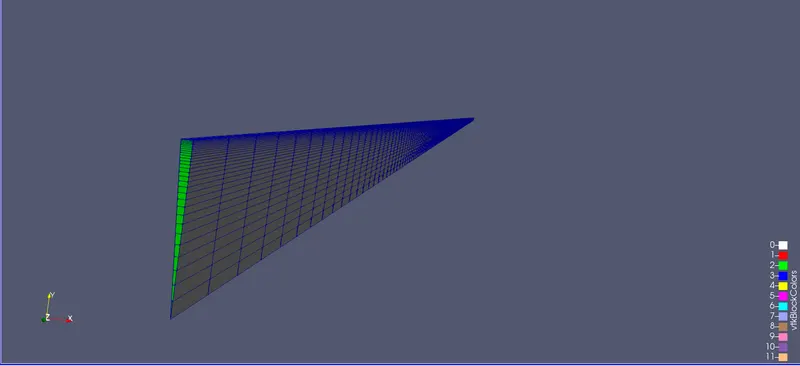
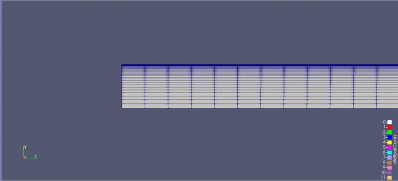
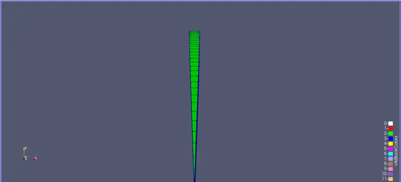
Following is the velocity and pressure boundary condition which is been updated according to the above-mentioned details. The velocity and pressure files are present in the zero (0) folder inside the constant folder.
The velocity and pressure boundary condition are can be seen below:
Velocity (U) field files:
/*--------------------------------*- C++ -*----------------------------------*\
  =========                 |
  \\      /  F ield         | OpenFOAM: The Open Source CFD Toolbox
   \\    /   O peration     | Website:  https://openfoam.org
    \\  /    A nd           | Version:  8
     \\/     M anipulation  |
\*---------------------------------------------------------------------------*/
FoamFile
{
    version     2.0;
    format      ascii;
    class       volVectorField;
    object      U;
}
// * * * * * * * * * * * * * * * * * * * * * * * * * * * * * * * * * * * * * //

dimensions      [0 1 -1 0 0 0 0];

internalField   uniform (0 0 0);

boundaryField
{
    inlet
    {
        type            fixedValue;
        value           uniform (0 0 0.1);
    }

    outlet
    {
        type            zeroGradient;
    }

    fixedWalls
    {
        type            noSlip;
    }

    front
    {
        type            wedge;
    }

    back
    {
        type            wedge;
    }

    bottom
    {
        type            empty;
    }
}

// ************************************************************************* //
Pressure (P) field files:
/*--------------------------------*- C++ -*----------------------------------*\
  =========                 |
  \\      /  F ield         | OpenFOAM: The Open Source CFD Toolbox
   \\    /   O peration     | Website:  https://openfoam.org
    \\  /    A nd           | Version:  8
     \\/     M anipulation  |
\*---------------------------------------------------------------------------*/
FoamFile
{
    version     2.0;
    format      ascii;
    class       volScalarField;
    object      p;
}
// * * * * * * * * * * * * * * * * * * * * * * * * * * * * * * * * * * * * * //

dimensions      [0 2 -2 0 0 0 0];

internalField   uniform 0;

boundaryField
{
    inlet
    {
        type            zeroGradient;
    }

    outlet
    {
        type            fixedValue;
        value		 uniform 0;
    }

    fixedWalls
    {
        type            zeroGradient;
    }

    front
    {
        type            wedge;
    }

    back
    {
        type            wedge;
    }

    bottom
    {
        type            empty;
    }
}

// ************************************************************************* //
Transproperties field files:
/*--------------------------------*- C++ -*----------------------------------*\
  =========                 |
  \\      /  F ield         | OpenFOAM: The Open Source CFD Toolbox
   \\    /   O peration     | Website:  https://openfoam.org
    \\  /    A nd           | Version:  8
     \\/     M anipulation  |
\*---------------------------------------------------------------------------*/
FoamFile
{
    version     2.0;
    format      ascii;
    class       dictionary;
    location    "constant";
    object      transportProperties;
}
// * * * * * * * * * * * * * * * * * * * * * * * * * * * * * * * * * * * * * //

nu              [0 2 -1 0 0 0 0] 0.000001;


// ************************************************************************* //
ControlDict file:
/*--------------------------------*- C++ -*----------------------------------*\
  =========                 |
  \\      /  F ield         | OpenFOAM: The Open Source CFD Toolbox
   \\    /   O peration     | Website:  https://openfoam.org
    \\  /    A nd           | Version:  8
     \\/     M anipulation  |
\*---------------------------------------------------------------------------*/
FoamFile
{
    version     2.0;
    format      ascii;
    class       dictionary;
    location    "system";
    object      controlDict;
}
// * * * * * * * * * * * * * * * * * * * * * * * * * * * * * * * * * * * * * //

application     icoFoam;

startFrom       startTime;

startTime       0;

stopAt          endTime;

endTime         50;

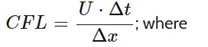
deltaT          0.001;

writeControl    timeStep;

writeInterval   20;

purgeWrite      0;

writeFormat     ascii;

writePrecision  6;

writeCompression off;

timeFormat      general;

timePrecision   6;

runTimeModifiable true;


// ************************************************************************* //
The end time and the deltaT values were calculated by the courant number formula.
After putting all these values, the simulation was run and the following results were obtained:
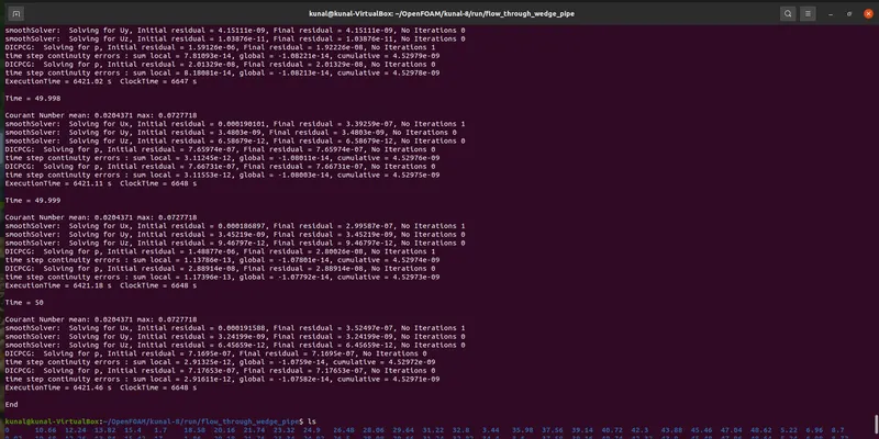
The above figure gives the result at the end of the simulation:
Simulation Time – 50 sec
Total clock time – 6648 sec
RESULTS:
After the simulation the pressure and velocity at the entrance and exit of the pipe are shown below:
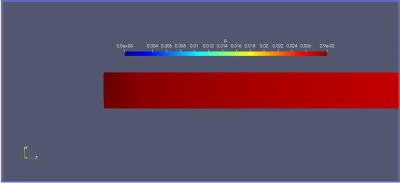
Fig: Pressure at the entrance of the pipe
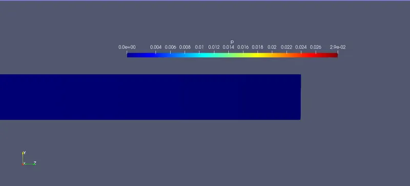
Fig: Pressure at the exit of the pipe
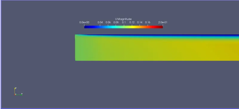
Fig: Velocity at the entrance of the pipe
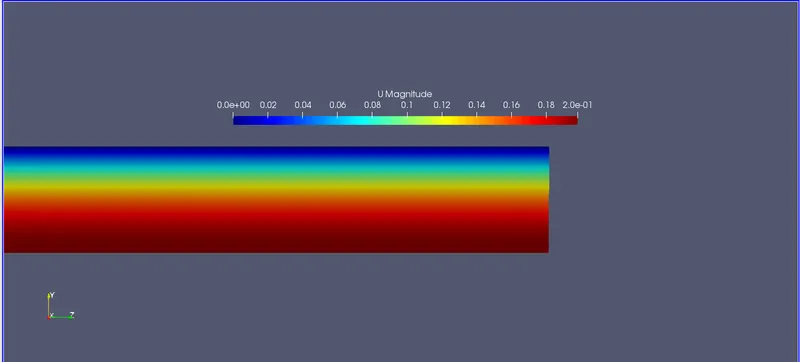
Fig: Velocity at the exit of the pipe
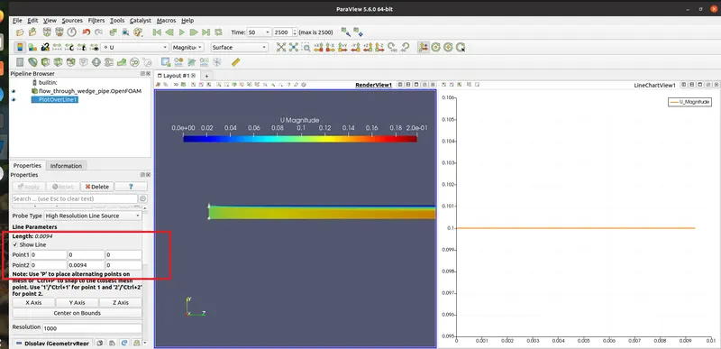
As these contour plots give very little explanation about the results, the plot over line command is used to get the line graph of velocity and pressure contour.
The graphs are shown below:
Velocity plot at the entrance:
Velocity plot at the exit:
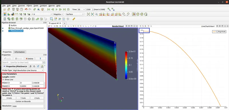
The above graphs explain how over the length of the pipe the velocity profile is developed and the steady-state fully developed laminar flow is obtained at the exit of the pipe.
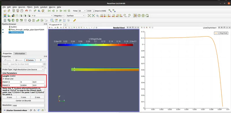
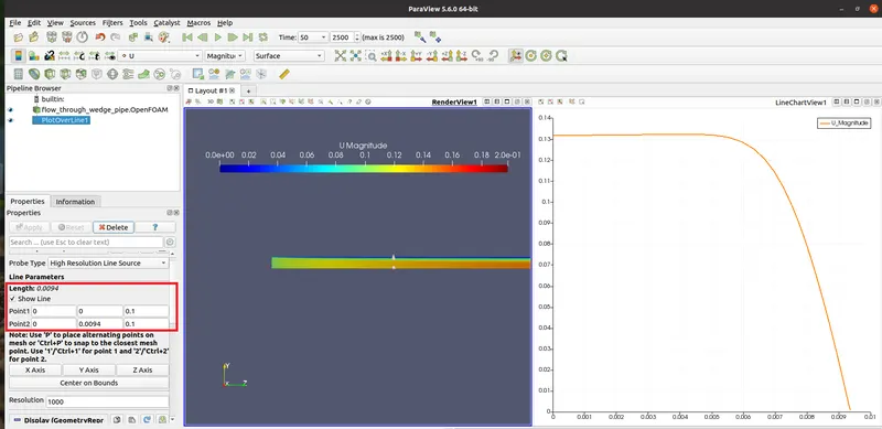
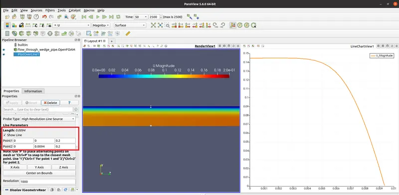
The following figure demonstrates the velocity profile development as the flow progresses over the length of the pipe:
At a distance of 0.01 m from the entrance:
At a distance of 0.1 m from the entrance:
At a distance of 0.2 m from the entrance:
At Exit:
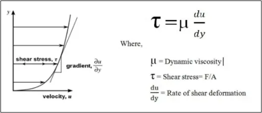
Further, the shear stress developed can be found out by using the following formula:
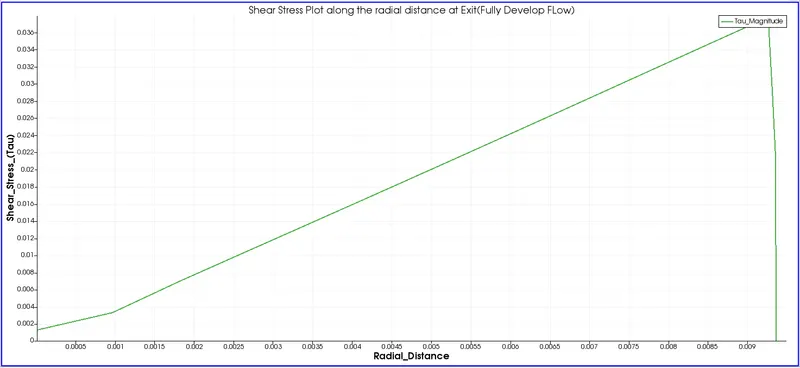
The below graph is obtained from the Para Foam window, the below link provides a detailed explanation of how the shear plot is obtained.
Link - https://skill-lync.com/knowledgebase/how-to-create-shear-stress-plot-inside-paraview
CONCLUSION:
- The HP equation was dully tested in this challenge as can be seen in the velocity plot of the pipe at the end of the pipe near the outlet.
- At x = 0.01 the velocity was seen slow and stable near the center of the pipe.
- Further, it can be seen that the flow starts to develop with an increase in length the profile becomes parabolic and a fully developed flow can be seen at the exit of the pipe.
- The MATLAB program was successfully developed for generating the blockMeshDict file and was successfully executed and the data processing between MATLAB and OpenFOAM was developed and understood.
- The shear stress plot also testifies the HP equation and the law for a fully developed region.
- The shear stress increases the friction at the wall of the pipe hence the minimum velocity is observed at the boundaries of the pipe and maximum at the center of the pipe.