week-11 Joint creation and Demonstration
Objective:
To illustrate the mechanism of spherical, cylindrical, translational and revolute joints between rigid bodies and deformable bodies.
The various types of joints can be created in LS-Dyna using the CONSTRAINED_JOINT keyword.
1. Joints between rigid bodies
The various types of joints between rigid bodies can be created in LS-Dyna using the CONSTRAINED_EXTRA_NODES keyword.
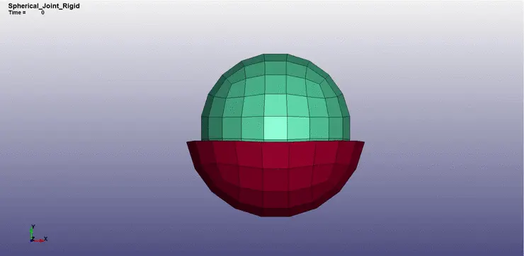
Spherical joint
The first step is to create two spherical bodies in LS-Dyna using the Entity option under Shape mesher in Element and mesh, and choosing spherical shell. The upper elements of the outer shell are deleted in order to get the required shape.
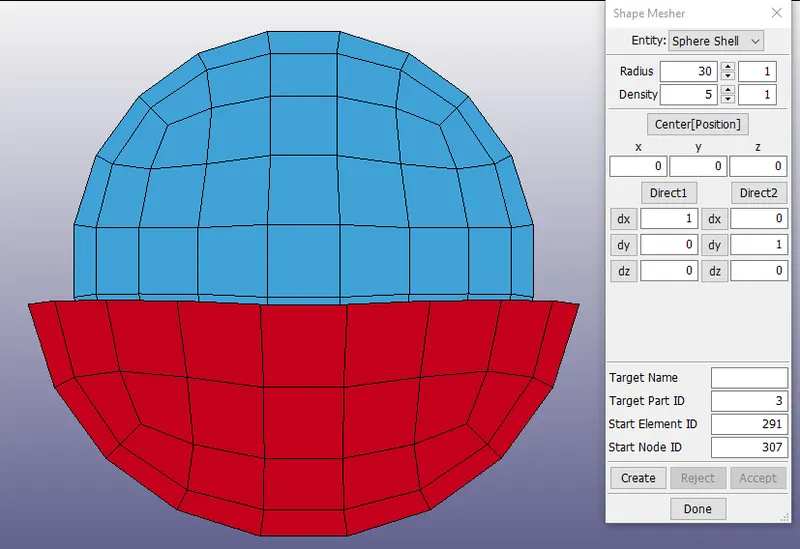
The material and section for the spheres are assigned as shown below
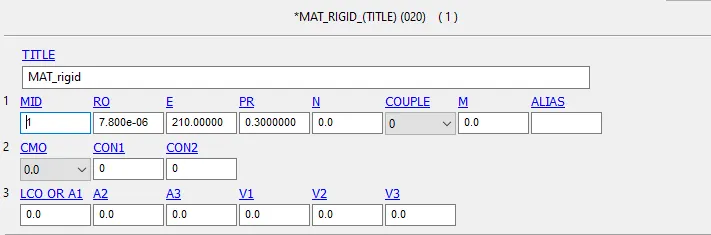
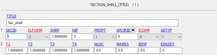
The same material and section properties are used for all the other types of joints.
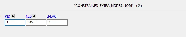
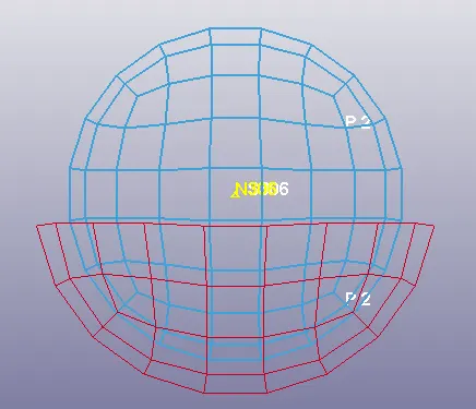
Two nodes are created for constraining, using Node edit option under Element Tools. The first node (305) is constrained to part 1, and the second node (306) is constrained to part 2. using CONSTRAINED_EXTRA_NODES, as shown below
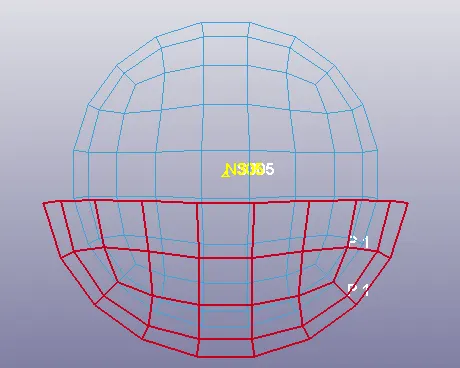

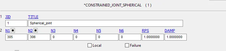
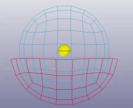
A spherical joint is then created between them, using the CONSTRAINED_JOINT menu.
An initial velocity of 20 mm/ms is applied to the part 2 (inner sphere), in all three rotational directions.

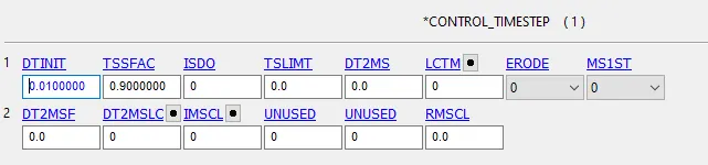
The simulation is set to run for 5 ms, and DTINIT is given as 0.01 ms.

The model is ready to run, and the results of the simulation can be viewed.
Revolute joint
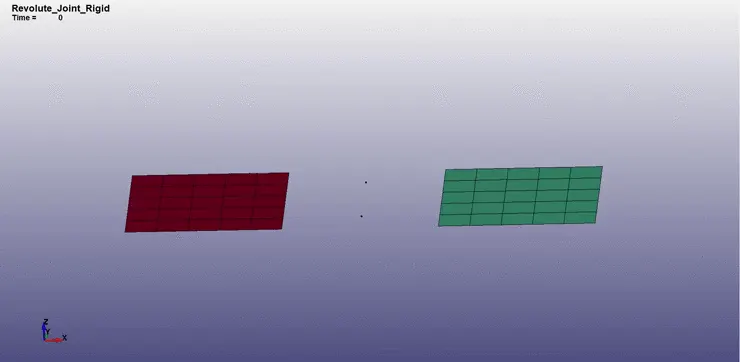
The first step is to create two bodies in LS-Dyna using the Entity option under Shape mesher in Element and mesh, and choosing 4N shell.
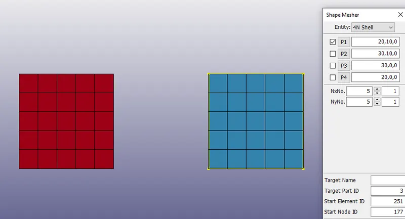
The material and section properties are the same as that of the spherical joint.
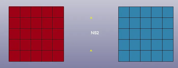
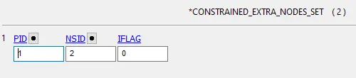
Two pairs of nodes are created for constraining, using Node edit option under Element Tools. The nodes 101, 103 are constrained to part 1 and 102,104 to part 2 respectively, using CONSTRAINED_EXTRA_NODES card. as shown below.
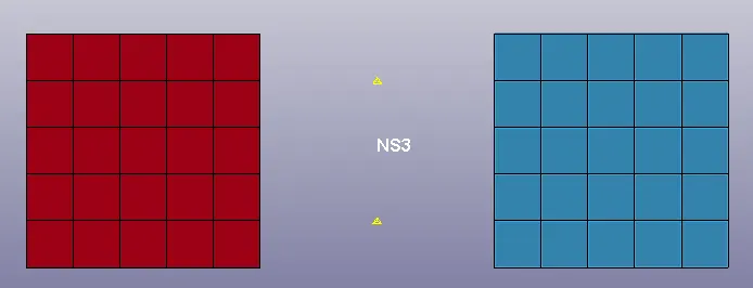

A revolute joint is then created between them, using the CONSTRAINED_JOINT menu, using nodes N1 and N3 of part 1 and N2,N4 of part 2.
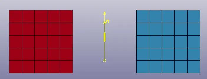
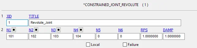
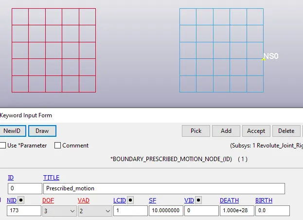
Part 1 (red) is fixed, and part 2 (blue) is the moving part. The part 1 is fixed with SPC's at all nodes, in order to prevent motion, and a prescribed motion is given to part 2, as shown below.
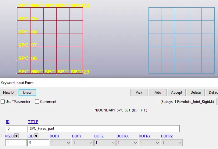
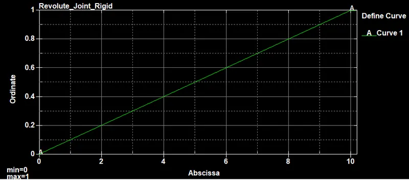
A load curve is defined with the required dispacement, and assigned to the LCID above.
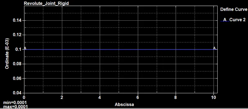
The control timestep is defined using the above timestep curve in the LCTM, and the termination time is given as 10 ms.
3. Cylindrical Joint
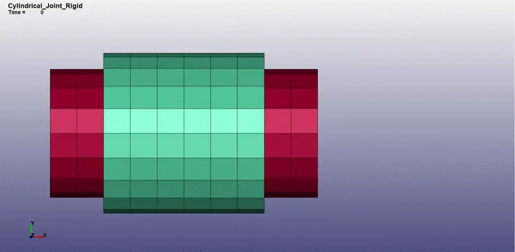
The first step is to create two bodies in LS-Dyna using the Entity option under Shape mesher in Element and mesh, and choosing cylinder shell.
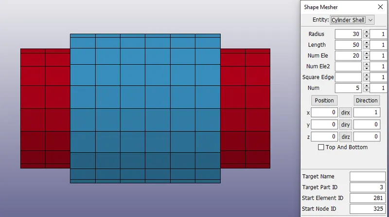
The material and section properties are the same as that of the spherical joint.
Two pairs of nodes are created for constraining, using Node edit option under Element Tools. The nodes 321, 323 are constrained to part 1 and 322,324 to part 2 respectively, using CONSTRAINED_EXTRA_NODES card, as shown below.
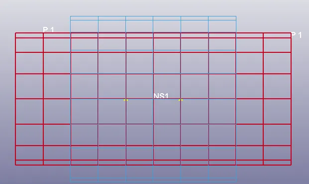

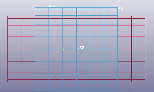
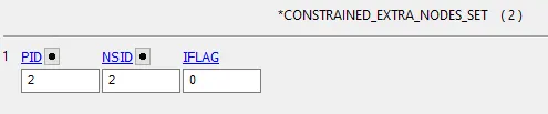
A cylindrical joint is then created between them, using the CONSTRAINED_JOINT menu, using nodes N1 and N3 of part 1 and N2,N4 of part 2
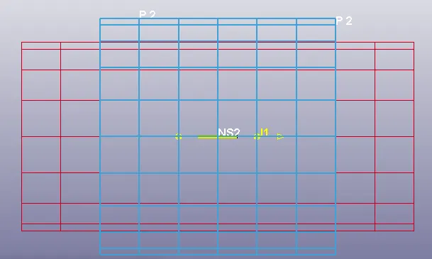
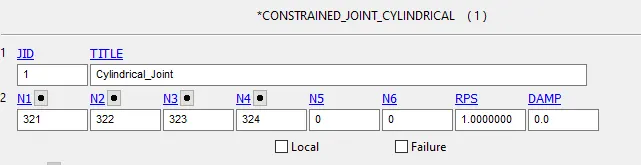
Part 2 (blue) is fixed, and part 1(red) is the moving part. An initial velocity of 10 mm/ms is given to part 1 in the x(translational) direction.

The simulation is set to run for 5 ms, and DTINIT is given as 0.01 ms.
The model is ready to run, and the results of the simulation can be viewed.
4. Translational Joint
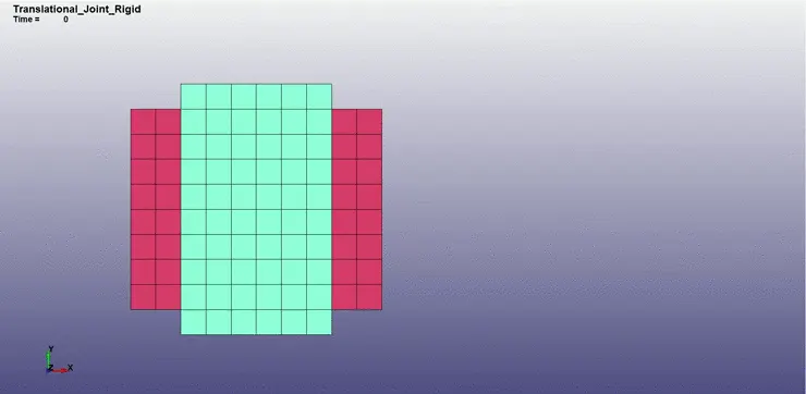
The first step is to create two bodies in LS-Dyna using the Entity option under Shape mesher in Element and mesh, and choosing box shell.
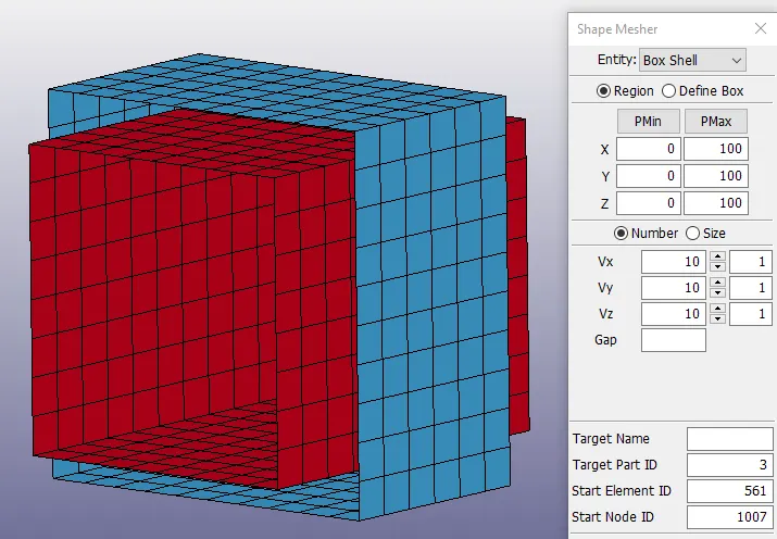
The material and section properties are the same as that of the spherical joint.
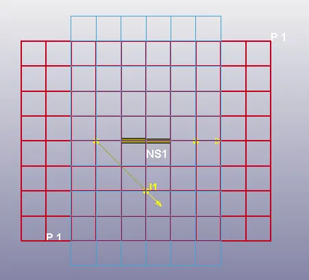
Three pairs of nodes are created for constraining, using Node edit option under Element Tools. The node pairs 1001,1002 and 1003,1004 are coincident and collinear. The third pair 1005,1006 is coincident, and slightly away from the axis of the other two pairs, in between them. The nodes 1001,1003 and 1005 are constrained to part 1 and 1002,1004 and 1006 to part 2 respectively, using CONSTRAINED_EXTRA_NODES card, as shown below.
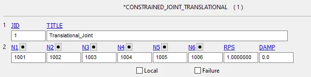
A translational joint is then created between them, using the CONSTRAINED_JOINT menu, using nodes N1,N3 and N5 of part 1 and N2,N4 and N6 of part 2, as shown above.
Part 2 (blue) is fixed, and part 1(red) is the moving part. An initial velocity of 10 mm/ms is given to part 1 in the x(translational) direction.
The simulation is set to run for 5 ms, and DTINIT is given as 0.01 ms.
The model is ready to run, and the results of the simulation can be viewed.
2. Joints between deformable bodies
The various types of joints between deformable bodies can be created in LS-Dyna using the CONSTRAINED_NODAL_RIGID_BODY keyword.
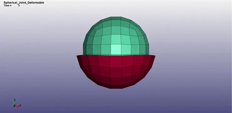
Spherical Joint
The first step is to create two spherical bodies in LS-Dyna using the Entity option under Shape mesher in Element and mesh, and choosing spherical shell. The upper elements of the outer shell are deleted in order to get the required shape.
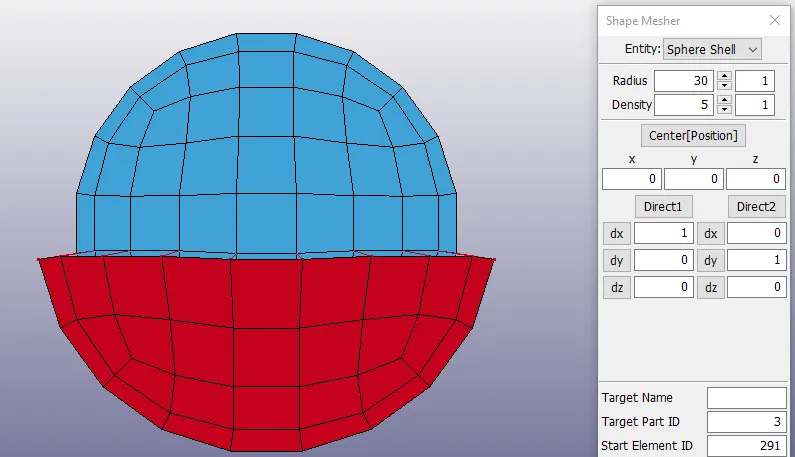
The material and section properties are the same as that of the rigid spherical joint.
The CNRB option is used between the peripheral nodes of the outer and inner hemispheres, for connecting them.
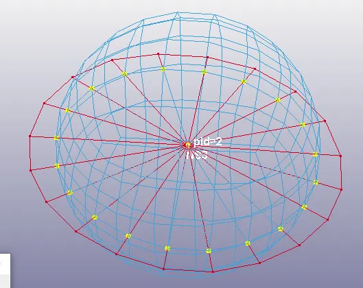
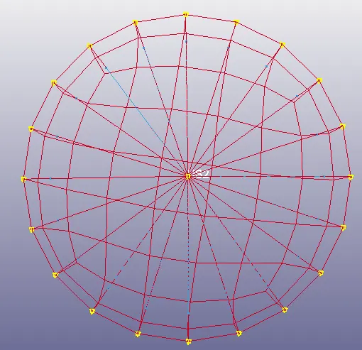
A spherical joint is then created between them, using the CONSTRAINED_JOINT menu.The first node (305) is constrained to part 1, and the second node (306) is constrained to part 2.
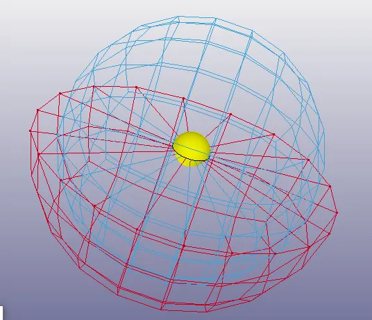
An initial velocity of 20 mm/ms is applied to the part 2 (inner sphere), in all three rotational directions.
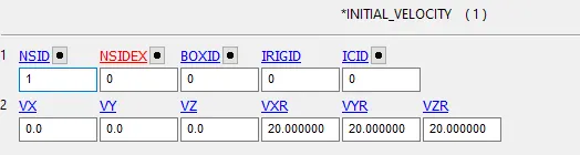
The simulation is set to run for 5 ms, and DTINIT is given as 0.01 ms.
The model is ready to run, and the results of the simulation can be viewed.
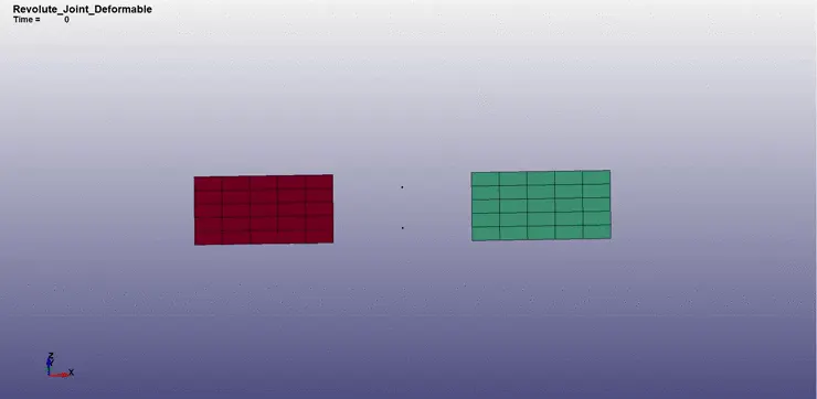
Revolute Joint
Revolute joint
The first step is to create two bodies in LS-Dyna using the Entity option under Shape mesher in Element and mesh, and choosing 4N shell.
The material and section properties are the same as that of the spherical joint.
Two pairs of nodes are created for constraining, using Node edit option under Element Tools. The nodes 101, 103 are constrained to part 1 and 102,104 to part 2 respectively, using CONSTRAINED_NODAL_RIGID_BODIES card.
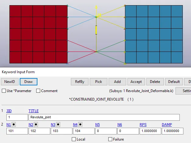
A revolute joint is then created between them, using the CONSTRAINED_JOINT menu, using nodes N1 and N3 of part 1 and N2,N4 of part 2.
Part 1 (red) is fixed, and part 2 (blue) is the moving part. The part 1 is fixed with SPC's at all nodes, in order to prevent motion, and a prescribed motion is given to part 2, similar to the rigid revolute joint.
A load curve is defined with the required dispacement, and assigned to the LCID above.
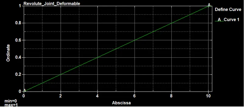
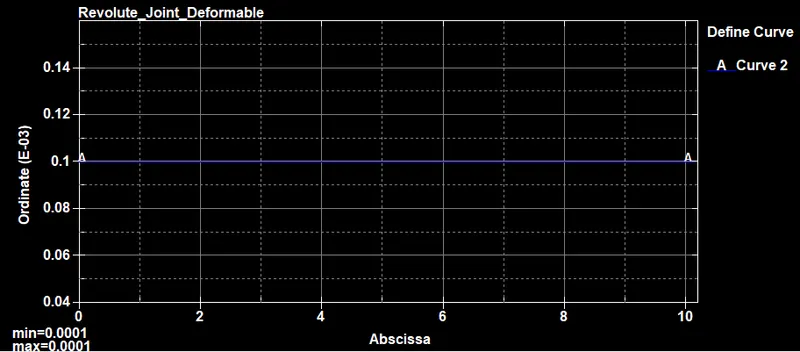
The control timestep is defined using the above timestep curve in the LCTM, and the termination time is given as 10 ms.
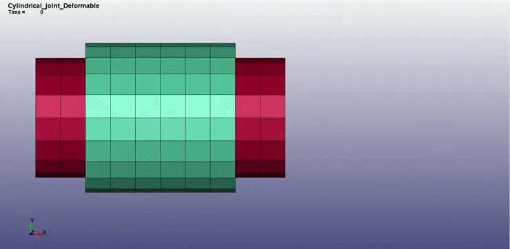
3. Cylindrical Joint
The first step is to create two bodies in LS-Dyna using the Entity option under Shape mesher in Element and mesh, and choosing cylinder shell.
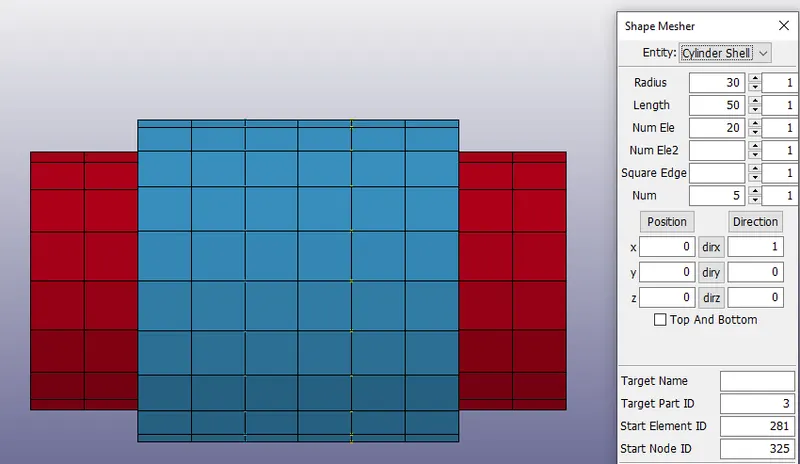
The material and section properties are the same as that of the spherical joint.
Two pairs of nodes are created for constraining, using Node edit option under Element Tools. The nodes 321, 323 are constrained to part 1 and 322,324 to part 2 respectively, using CONSTRAINED_NODAL_RIGID_BODY card, as shown below.
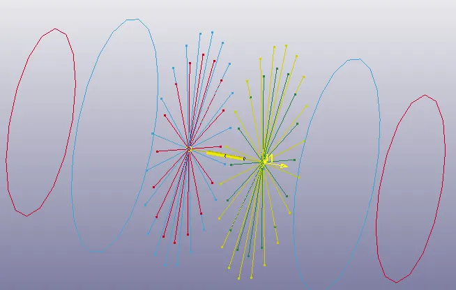
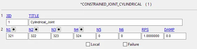
A cylindrical joint is then created between them, using the CONSTRAINED_JOINT menu, using nodes N1 and N3 of part 1 and N2,N4 of part 2.
Part 2 (blue) is fixed, and part 1(red) is the moving part. An initial velocity of 10 mm/ms is given to part 1 in the x(translational) direction.
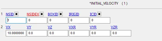
The simulation is set to run for 5 ms, and DTINIT is given as 0.01 ms.
The model is ready to run, and the results of the simulation can be viewed.
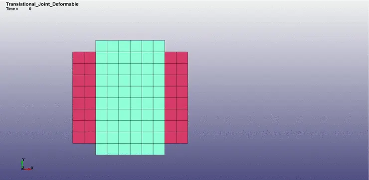
Translational Joint
The first step is to create two bodies in LS-Dyna using the Entity option under Shape mesher in Element and mesh, and choosing box shell.
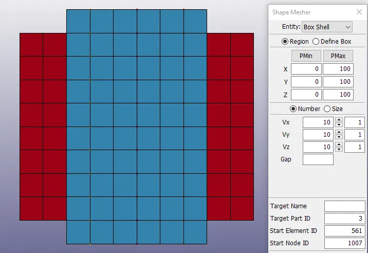
The material and section properties are the same as that of the spherical joint.
Three pairs of nodes are created for constraining, using Node edit option under Element Tools. The node pairs 1001,1002 and 1003,1004 are coincident and collinear. The third pair 1005,1006 is coincident, and slightly away from the axis of the other two pairs, in between them. The nodes 1001,1003 and 1005 are constrained to part 1 and 1002,1004 and 1006 to part 2 respectively, using CONSTRAINED_NODAL_RIGID_BODIES card, as shown below.
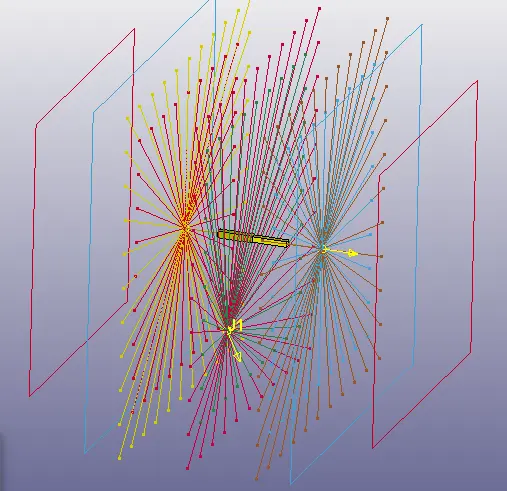
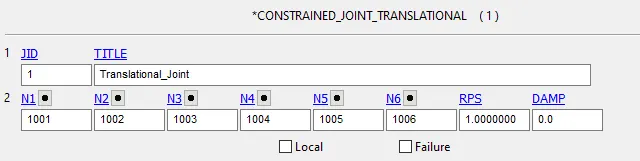
A translational joint is then created between them, using the CONSTRAINED_JOINT menu, using nodes N1,N3 and N5 of part 1 and N2,N4 and N6 of part 2, as shown above.
Part 2 (blue) is fixed, and part 1(red) is the moving part. An initial velocity of 10 mm/ms is given to part 1 in the x(translational) direction.
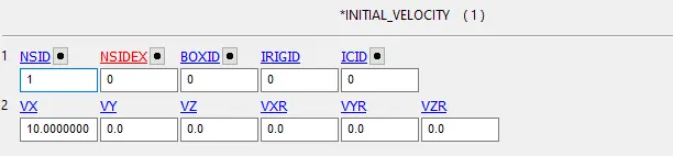
The simulation is set to run for 5 ms, and DTINIT is given as 0.01 ms.
The model is ready to run, and the results of the simulation can be viewed.
Results
1. Rigid bodies
Spherical Joint
Revolute Joint
Cylindrical Joint
Translational Joint
1. Deformable bodies
Spherical Joint
Revolute Joint
Cylindrical Joint
Translational Joint
Conclusion
Thus the various joints are created and studied between rigid and deformable bodies, and the results of the simulation have been illustrated.