Joint creation and Demonstration in LS-Dyna

OBJECTIVE

• To represent joints modeling in ls-dyna, for rigid and deformable bodies.

SPHERICAL JOINT BETWEEN RIGID BODIES

When two groups of elements are connected in such a way that one group swivel about the other group of elements, such a pair is called a spherical joint. The side mirror of a bike, tie rod ends of the steering system, pen stand, are some examples of it.

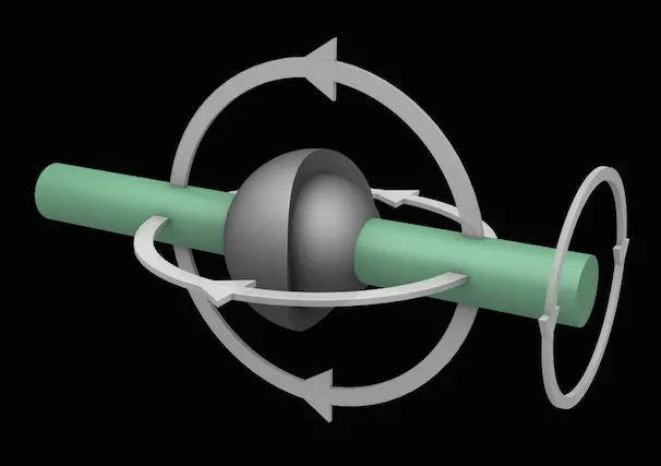
Figure 1: Spherical Joint. (Image source: www.xemo.io/edu/robot/actuators/)

Using Element and mesh → Shape Mesher, two spheres were modeled as required for the spherical joint. Elements of the upper half of the outer sphere were deleted to give it a socket-type shape. The outer sphere was given a radius of 30 mm, and the inner sphere was given a radius of 25 mm.

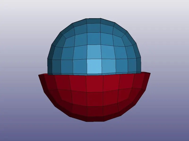
Figure 2: Inner sphere and outer hemisphere representing the ball and socket, modeled in LS-Dyna.

After creating the two parts, a material card had to be assigned to it. Thus, a material card with steel material property was created.

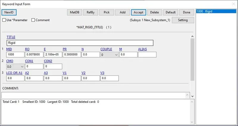
Figure 3: Material Card for the ball and socket.

Also, a section was required. Thus, the *SECTION_SHELL card was created to give the thickness of 1 mm to the shell elements.

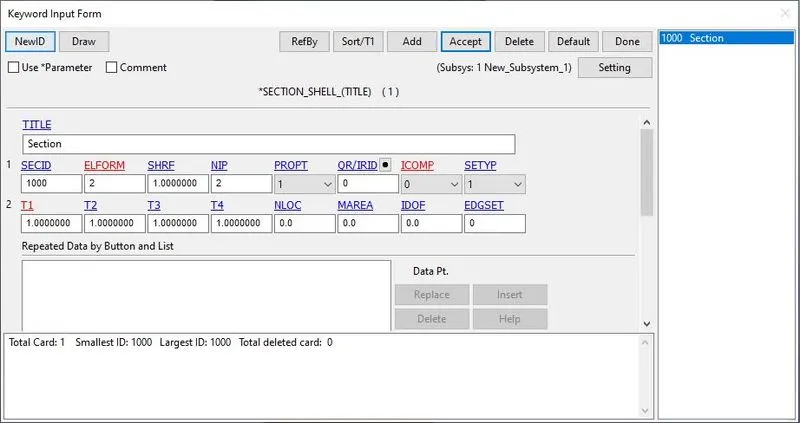
Figure 4: *SECTION_SHELL card to give the thickness of 1 mm.

Using Element Tools → Node Editing → Create, two separate central nodes were created for both ball and socket.

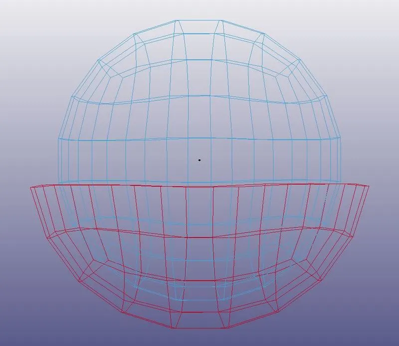
Figure 5: Two central nodes created for two spheres.

It was then, constrained to their respective spheres, viz. one central node to the ball, and one central node to the socket, using *CONSTRAINED_EXTRA_NODES_NODE card.

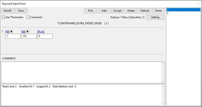
Figure 6: The central node was constrained to the sphere. Central node 153 to the ball, and central node 154 to the socket.

Then, using *CONSTRAINED_JOINT_SPHERICAL, the two central nodes were used to create the rigid spherical joint between the ball and socket.

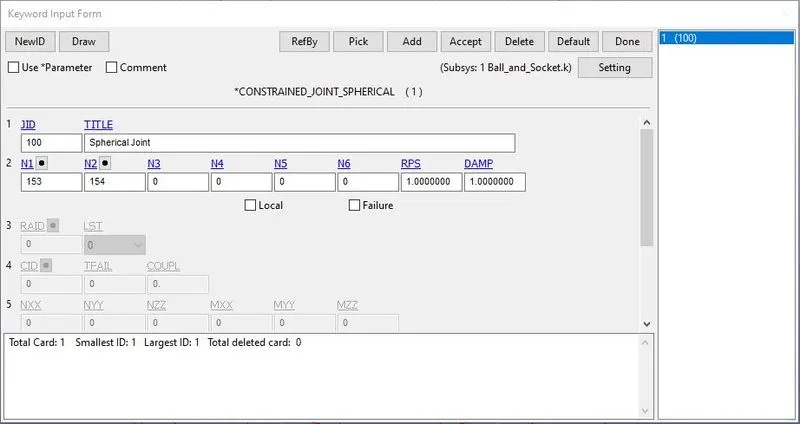
Figure 7: *CONSTRAINED_JOINT_SPHERICAL card to create a spherical joint.

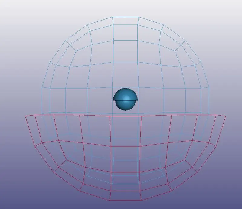
Figure 8: Spherical joint created between two spheres.

Once everything required was modeled, then, the socket was given an initial rotational velocity, to check its working. It was accomplished using *INITIAL_VELOCITY_RIGID_BODY card.

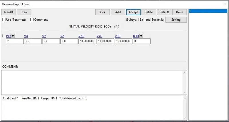
Figure 9: *INITIAL_VELOCITY_RIGID_BODY card to give the initial rotational velocity to the socket, to check the joint creation.

A *CONTROL_TERMINATION card was created to simulate 5 ms. A *CONTROL_TIMESTEP card was also used to give the initial time step of 0.01 ms. The problem was solved and, in the simulation, the joint creation had to check, which was found to be as expected.

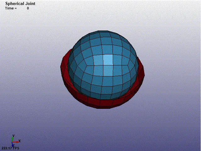
Figure 10: Spherical joint for rigid bodies.

REVOLUTE JOINT BETWEEN RIGID BODIES

When the two groups of elements are connected in such a way that one group can revolve about a fixed axis, such a joint is called a revolute joint.

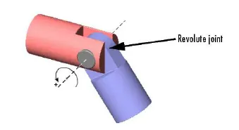
Figure 11: Revolute Joint

(Image source: https://www.researchgate.net/publication/228687250_Dynamic_balancing_of_linkages_by_algebraic_methods)

To demonstrate the revolute joint in ls-dyna, two plates of 5x5 shell elements were created, as shown in the figure below.

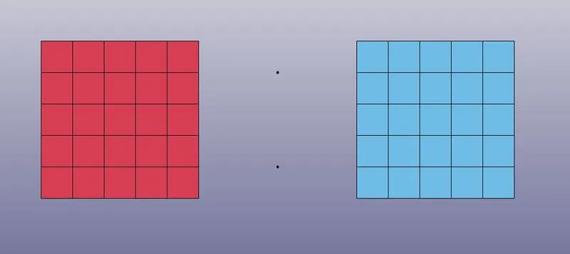
Figure 12: Two plates with 5x5 shell elements, with pair of central nodes.

Similar to the case in the spherical joint, in this case also, the *MAT_RIGID material and *SECTION_SHELL section cards were applied to shell elements.

Two pairs of nodes were created in the middle of the plates. Each pair was constrained to each plate respectively. In other words, nodes with node id 73 and 74 were constrained to the red plate, and nodes with node ids 75 and 76 were constrained to the blue plate, using *CONSTRAINED_EXTRA_NODES_NODE card.

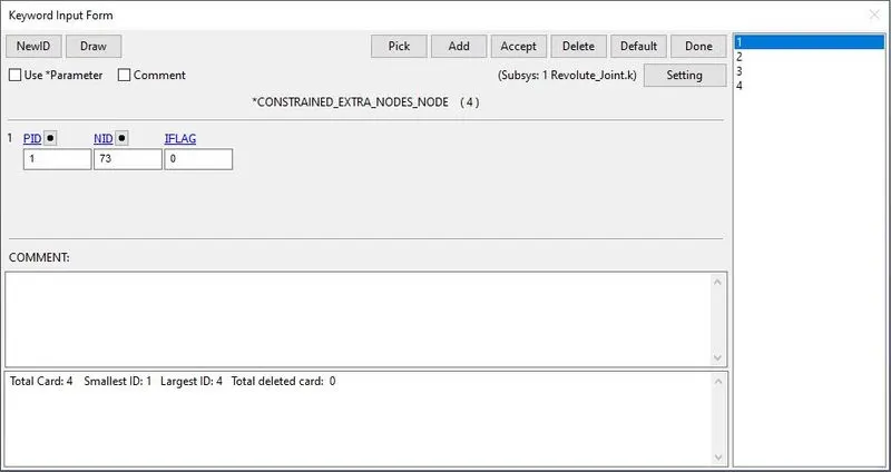
Figure 13: *CONSTRAINED_EXTRA_NODES_NODE card to constrain the pair of central nodes to each plate.

After modeling the parts, *CONSTRAINED_JOINT_REVOLUTE card was used to create a revolute joint between these two plates. In this card, N1, and N3 are the nodes from plate A, and N2, and N4 are the nodes from plate B.

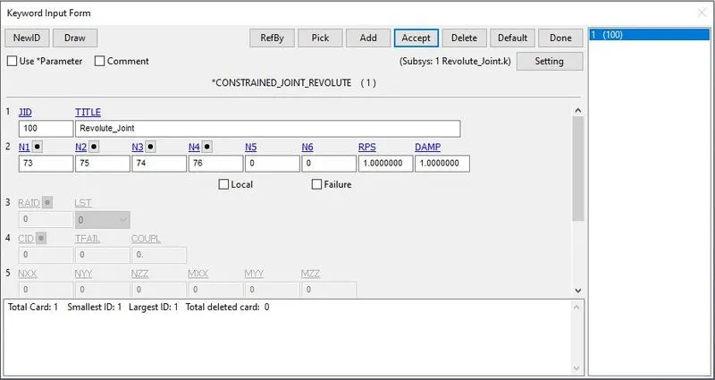
Figure 14: *CONSTRAINED_JOINT_REVOLUTE card was used to create a revolute joint.

To check whether the joint is correctly applied or not, it had to analyze. Thus, a boundary condition was used, in which, using *BOUNDARY_SPC_SET, all the nodes of red plates were fixed in all directions.

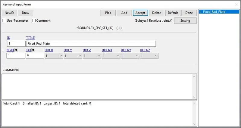
Figure 15: Red plate was fixed in all directions.

Then, a displacement curve was created, which was then used to apply the motion to one node of the blue plate, using *BOUNDARY_PRESCRIBED_MOTION_NODE card.

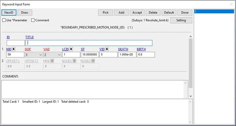
Figure 16: *BOUNDARY_PRESCRIBED MOTION_NODE card was used to apply motion to the free blue plate.

To run the simulation, a constant timestep was applied by defining a curve as shown below.

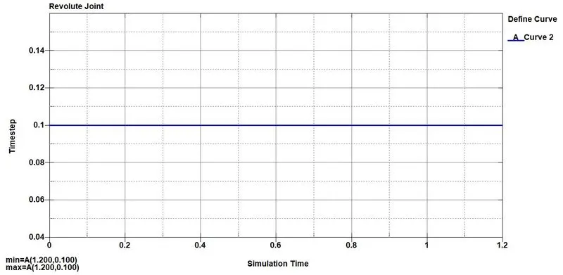
Figure 17: Constant timestep during simulation.

Similar to the spherical joint case, the *CONTROL_TERMINATION card was used to simulate 10 ms. A *CONTROL_TIMESTEP card was used to give the initial time step of 0.01 ms, and the timestep curve, i.e., shown in fig.17, was applied. The problem was solved and, in the simulation, the joint creation had to check, which was found to be as expected.

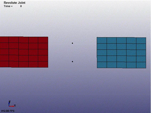
Figure 18: Revolute joint for rigid bodies.

CYLINDRICAL JOINT BETWEEN RIGID BODIES

When two groups of elements, in a cylindrical shape, have one common axis of rotation and are free to rotate and slide relative to each other, such a joint is called a cylindrical joint. To model such joint in ls-dyna, two cylindrical parts had to be model. Thus, using Element and mesh → Shape Mesher → Entity → Cylinder Shell, two cylindrical parts with a common axis were created. And similar to earlier cases, *MAT_RIGID material card and *SECTION_SHELL card were applied to it, with steel material property, and thickness of 1 mm respectively.

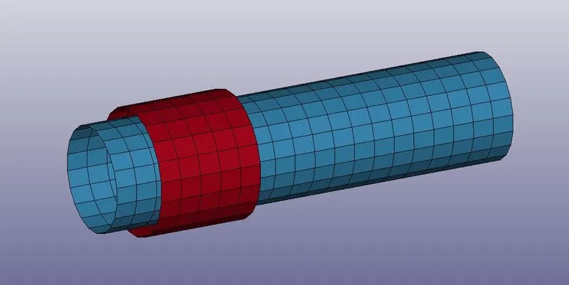
Figure 19: Two cylindrical parts with a common axis, modeled in ls-dyna.

Then, similar to the case of revolute joint, using the Element Tools → Node Editing → Create, 2 pair of nodes was created, to define common the axis of rotation. Using *CONSTRAINED_EXTRA_NODES_NODE, one pair was constrained to the red part, and the other pair was constrained to another part.

Then using *CONSTRAINED_JOINT_CYLINDRICAL card, the cylindrical joint was defined.

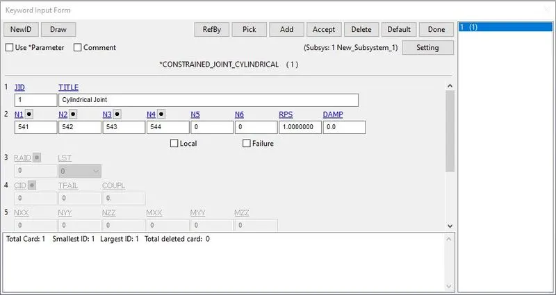
Figure 20: *CONSTRAINED_JOINT_CYLINDRICAL to define the cylindrical joint.

Once done with modeling the joint, now to check, if the joint was applied properly or not, an *INITIAL_VELOCITY_RIGID_BODY card was used. Using this card, the initial linear and rotation velocity of 10 units was applied in the x-direction, to the outer part.

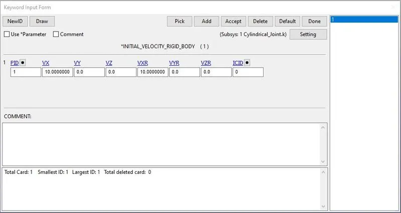
Figure 21: *INITIAL_VELOCITY_RIGID_BODY card was used to apply the initial velocity to the outer part.

Then, the *CONTROL_TERMINATION card was used to run the simulation for 10 ms. A *CONTROL_TIMESTEP card was also used to give the initial time step of 0.01 ms. The problem was solved and, in the simulation, the joint creation had to check, which was found to be as expected.

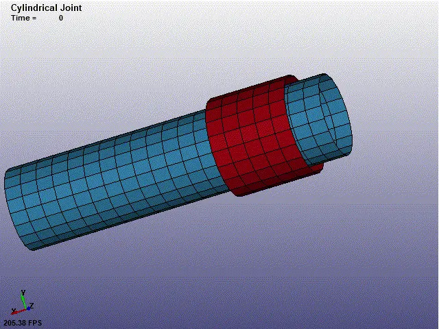
Figure 22: Cylindrical joint for rigid bodies.

TRANSLATIONAL JOINT BETWEEN RIGID BODIES

When two groups of elements have one common axis to slide over each other, such joint is called translational or sliding joint. To model such joint in ls-dyna, two tube parts with rectangular shapes had to model. Thus, using Element and mesh → Shape Mesher → Entity → Box Shell, two tube parts with a common axis were created. And similar to earlier cases, *MAT_RIGID material card and *SECTION_SHELL card were applied to it, with steel material property, and thickness of 1 mm respectively.

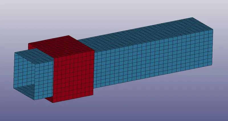
Figure 23: Translational joint with a common axis, modeled using ls-dyna.

Now, similar to earlier cases, using Element Tools → Node Editing → Create, two pairs of nodes had to create to define the axis. Along with this, while creating a translational joint, one more pair is required to define the plane of translation. It has to be slightly away from the axis, and the plane forming by three pairs of nodes should be parallel to the surface of the two parts. One pair of nodes can be seen in the figure below.

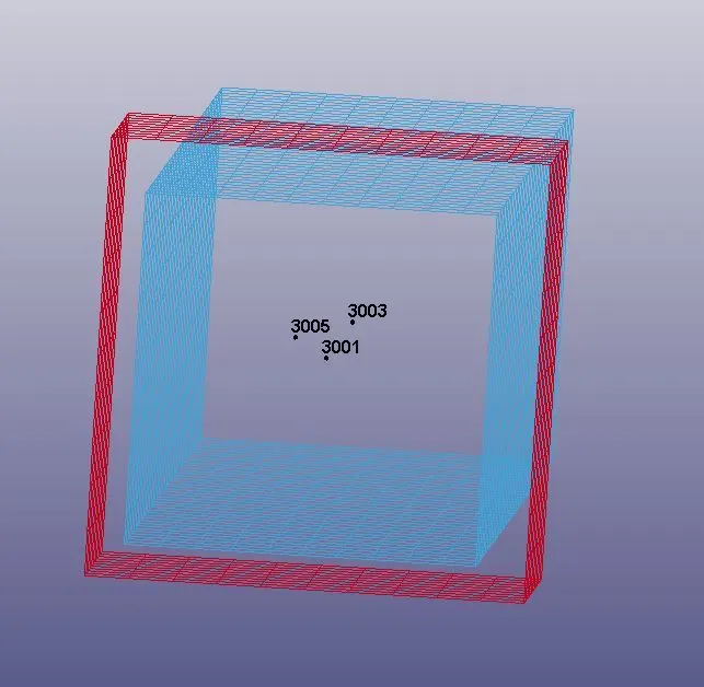
Figure 24: Three pairs of nodes are required to define the plane of translation.

Using *CONSTRAINED_EXTRA_NODES_NODE, one pair was constrained to the red outer part, and the other pair was constrained to the blue inner part. Now, using *CONSTRAINED_JOINT_TRANSLATIONAL, each of the pair of nodes was defined respectively to N1, N2, N3, N4, N5, and N6, and the joint was created.

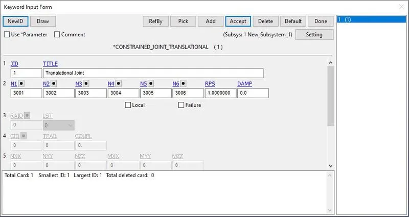
Figure 25: *CONSTRAINED_JOINT_TRANSLATIONAL card was used to create a translational joint.

To check the whether joint was properly created or not, an initial velocity was applied to the outer red part, using the *INITIAL_VELOCITY_RIGID_BODY card, and similar to earlier cases, the *CONTROL_TERMINATION card was used to run the simulation for 10 ms. A *CONTROL_TIMESTEP card was also used to give the initial time step of 0.01 ms. The problem was solved and, in the simulation, the joint creation had to check, which was found to be as expected.

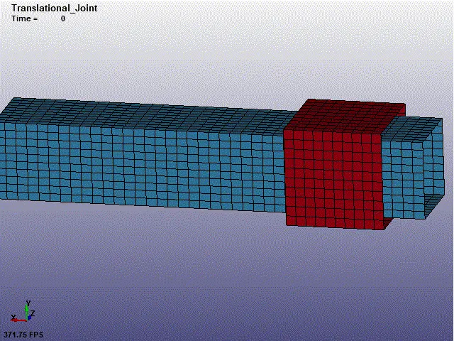
Figure 26: Translational joint for rigid bodies.

SPHERICAL JOINT BETWEEN DEFORMABLE BODIES

Similar to the case where the spherical joint was created for rigid material, in this case also, two spheres were created, but they were assigned with *MAT_ELASTIC material card instead of *MAT_RIGID card, with the material property of steel. The section card remained the same as before, i.e., *SECTION_SHELL, with 1 mm of shell thickness.

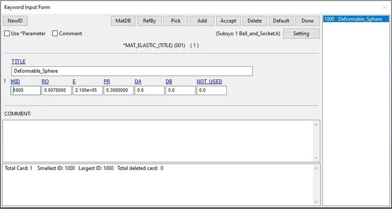
Figure 27: *MAT_ELASTIC card for the spheres.

Now, two central nodes were created, two for each sphere, as in the earlier cases. Instead of constraining them using *CONSTRAINED_EXTRA_NODES_NODE card, in case of deformable bodies, those two nodes are constrained to a sphere using Model and Part → Create Entity → Constrained → Nodal Rigid Body (CNRB). In that card, CrePNode was turned off, which takes the mass center as the first node. Instead, by turning it off now, the first node is considered as the central node. This is how the central node that was created earlier was assigned to the spheres. For example, in this work, for constraining the central node to the outer ball part, a node with node id 153 was selected first, and then the nodes of the ball part were selected. Similarly, for the inner socket part, a central node with node id 154 was selected first, and then the nodes of the socket were selected. This is how both spheres have their centers at the center and both the central nodes are coinciding.

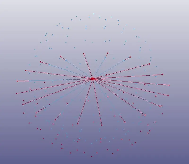
Figure 28: Central nodes constrained to spheres using constrained nodal rigid body (CNRB).

Now, as performed before, *CONSTRAINED_JOINT_SPHERICAL card was used, and the central nodes of two spheres were selected as nodes N1 and N2. This is how the joint was created. To check the creation of the joint, an initial velocity was given to the socket using an *INITIAL_VELOCITY card (not *INITIAL_VELOCITY_RIGID_BODY) and applied initial rotational velocity in all the directions.

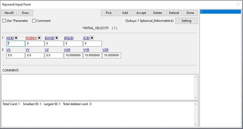
Figure 29: *INITIAL_VELOCITY card to give the initial velocity to the deformable socket part of the spherical joint.

A *CONTROL_TERMINATION card was created to run the simulation for 5 ms. A *CONTROL_TIMESTEP card was also used to give the initial time step of 0.01 ms. The problem was solved and, in the simulation, the joint creation had to check, which was found to be as expected. The simulation looks like fig. 10.

REVOLUTE JOINT BETWEEN DEFORMABLE BODIES

Similar to the joint created for rigid bodies, in this case also two plates were created with pair of central nodes for each plate, as shown in fig. 12. Instead of *MAT_RIGID, *MAT_ELATIC card was assigned to both the plates with the material property of steel. No change with the Section card. To constrain the pair of central nodes to the plates, in this case, instead of *CONSTRAINED_EXTRA_NODES_NODE card, Model and Part → Create Entity → Constrained → Nodal Rigid Body (CNRB) was used. Thus, using CNRB, the pair of central nodes were constrained to each plate.

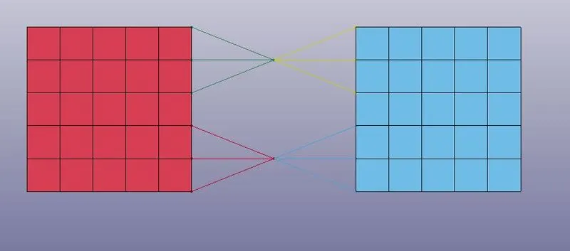
Figure 30: Pair of central nodes constrained to deformable plates using CNRB.

After modeling the parts, *CONSTRAINED_JOINT_REVOLUTE card was used to create a revolute joint between these two plates. In this card, N1, and N3 are the nodes from plate A (in this work, red plate), and N2, and N4 are the nodes from plate B (in this work, blue plate).

Now, as done before, one plate (red plate, in this work) is fixed using Model and Part → Create Entity → Boundary → Spc, in all directions. And using *BOUNDARY_PRESCRIBED_MOTION_NODE, a displacement is given to one node of the other plate (blue plate).

The *CONTROL_TERMINATION card was used to run the simulation for 10 ms. A *CONTROL_TIMESTEP was set as before (in the case of revolute joint for rigid bodies). The problem was solved and, in the simulation, the joint creation had to check, which was found to be as expected.

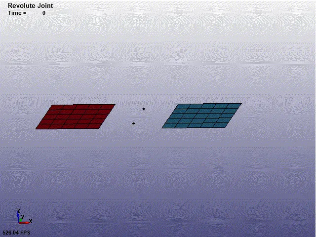
Figure 31: Revolute joint for deformable bodies.

CYLINDRICAL JOINT BETWEEN DEFORMABLE BODIES

For demonstrating the cylindrical joint for deformable bodies, two cylinders were created as before (fig. 19).

*MAT_ELASTIC was used, provided it the material property of steel, in (gm, mm, ms) unit, and assigned to both the cylinders. Then, *SECTION_SHELL card was used to define the thickness of 1 mm to both the cylinders.

To define the common axis of the cylinders, two pairs of central nodes were created with node ids 541, 542, 543, and 544. Using Model and Part → Create Entity → Constrained → Nodal Rigid Body (CNRB), each pair was constrained to each pair as shown in the figure below.

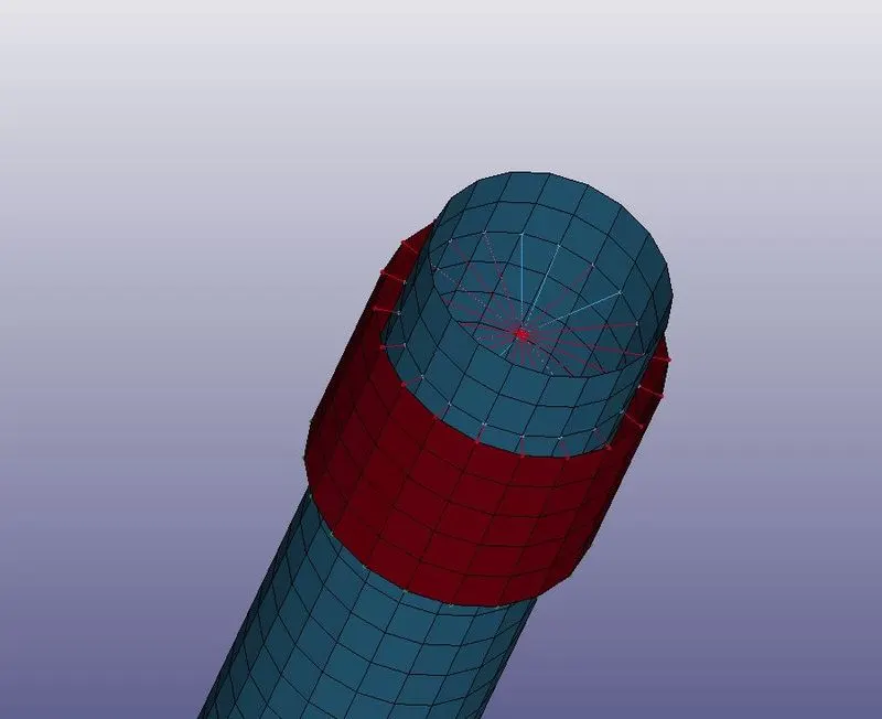
Figure 28: Pair of central nodes that were constrained to each cylinder.

Then, as shown in fig. 19, *CONSTRAINED_JOINT_CYLINDRICAL card was used to create a cylindrical joint between two cylinders. To check, if the joint was applied properly or not, an *INITIAL_VELOCITY card was used. Using this card, the initial linear and rotation velocity of 10 units was applied in the axial direction, to the node-set of the outer part.

Then, the *CONTROL_TERMINATION card was used to run the simulation for 10 ms. A *CONTROL_TIMESTEP card was also used to give the initial time step of 0.01 ms. The problem was solved and, in the simulation, the joint creation had to check, which was found to be as expected. The simulation looks like fig. 22.

TRANSLATIONAL JOINT BETWEEN DEFORMABLE BODIES

To demonstrate the translational joint for deformable bodies, two rectangular cylinders were created as shown in fig. 21. *MAT_ELASTIC was used, provided it the material property of steel, in (gm, mm, ms) unit, and assigned to both the rectangular cylinders. Then, *SECTION_SHELL card was used to define the thickness of 1 mm to both the cylinders.

To define the common axis and the plane of translation, three pairs of nodes were created for each rectangular cylinder, as shown in fig. 22. Two nodes on the central axis, and one slightly away from the axis. Then, using Model and Part → Create Entity → Constrained → Nodal Rigid Body (CNRB), each pair was constrained to each cylinder, as shown in the figure below.

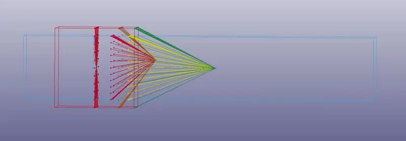
Figure 29: Pair of nodes constrained to each cylinder, using CNRB.

Now, similar to the case of joint for rigid bodies, using *CONSTRAINED_JOINT_TRANSLATIONAL, each of the pair of nodes was defined respectively to N1, N2, N3, N4, N5, and N6, and the joint was created.

To check that if the joint was properly created or not, an initial velocity was applied to the outer red part, using the *INITIAL_VELOCITY card. The *CONTROL_TERMINATION card was used to run the simulation for 10 ms. A *CONTROL_TIMESTEP card was also used to give the initial time step of 0.01 ms. The problem was solved and, in the simulation, the joint creation had to check, which was found to be as expected.

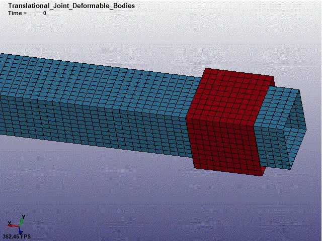
Figure 30: Translational Joint for Deformable Bodies

CONCLUSION

In this work, four kinds of joints were created for rigid bodies and deformable bodies. The joints were spherical, revolute, cylindrical, and translational. The joints work the same in both rigid and deformable cases, but the way of modeling the joint is different. Moreover, while simulating, the problem solves faster in the case of the rigid body, while in the case of a deformable body, it takes a bit longer. This can be because of more parameters to calculate in the case of deformable cases.