week-11 Joint creation and Demonstration

Joint Creating and Demonstration

Objective

• Create a revolute, spherical, cylindrical and translation joint between two rigid and two deformable bodies using LS-Dyna

Background

Mechanical joints play a vital role in various fields of engineering such as robotics, machine elements and even automotive/aerospace engineering. They enable connection and movement of different components and mechanisms. Each type of joint posses different characteristics that allow/restrain specific degrees of freedom to produce different types of motion. Some of the most common types of joints include:

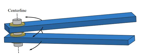
- Revolute/Hinge Joint: This type of joint enables rotational motion around a single axis. It usually consists of a cylinder and a pin-shaped connector that rotates relative to the frame. This type of joint can be found in door hinges, robotic arms and even in elbow/knee skeletal joints.

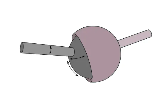
- Spherical Joint: This type of joint enables three rotational degrees of freedom with respect to the frame. It usually consists of a ball-shaped connector inside a socket. It can be found in vehicle suspensions, mechanical limbs and even in articulated robotic arms/mechanisms

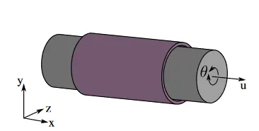
- Cylindrical Joint: This type of joint enables both linear and rotational motion around a single axis. It usually consists of a cylindrical connector inside a slot/sleeve. It can be found in sliding drawers and telescopic mechanisms

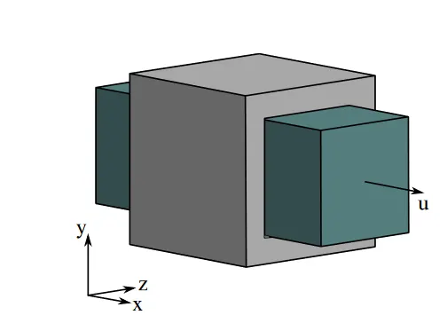
Translational Joint: This joint type is similar to the cylindrical joint, but it prevents the rotational degree of freedom around the axis. It can be found in several types of gantries

Procedure

Case 1) Revolute Joint between two rigid bodies

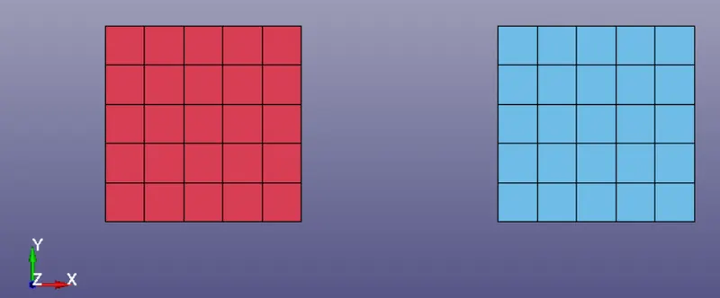
Starting by the revolute joint between rigid bodies, we will first use the Shape Mesher menu to create two shell elements with some separation between them.

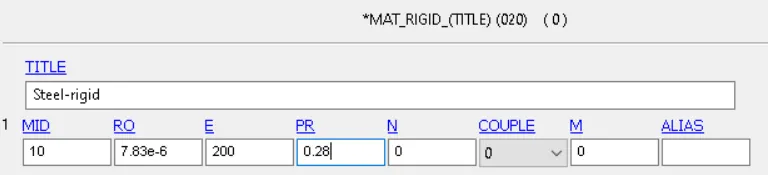
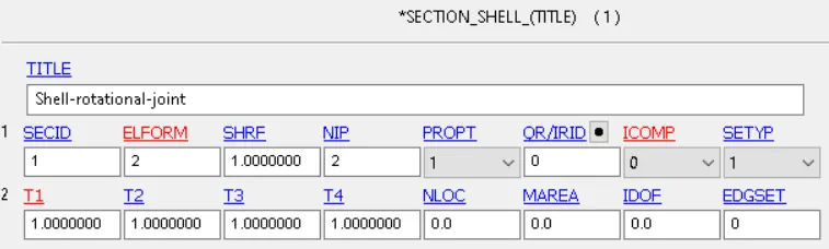
As in any other analysis, we also must define a rigid material (MAT020) and section properties to avoid errors during the simulation

Then, four extra nodes must be created manually. To do so, we simply must go to the Element tools ---> Node editing menu

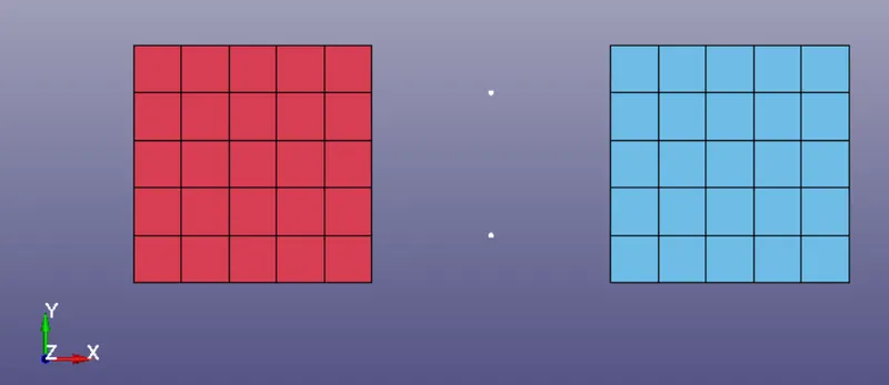
This pair of nodes (1001, 1003 and 1002, 1004) are then associated to the Shell 1 and 2 rigid parts using a Constrained extra node set keyword

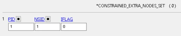
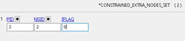
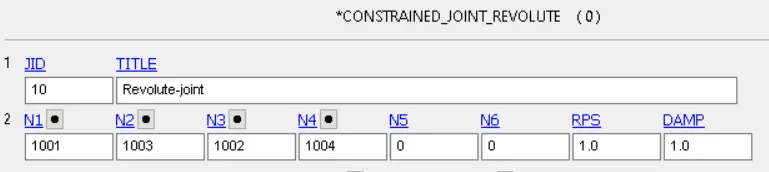
From there we can proceed to define the revolute joint behavior by using a Constrained Joint Revolute keyword. We must remember that nodes 1 and 3 must belong to the first body, and nodes 2 and 4 to the second one.

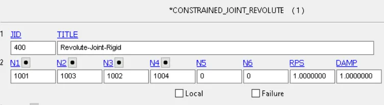
Lastly, some boundary conditions are required to demonstrate the joint behavior. In particular:

• Some edge nodes of the first part will be constrained in all DOF's to work as frame
• A node in the second part will be given a fixed displacement in the Z direction to perform the hinge motion

4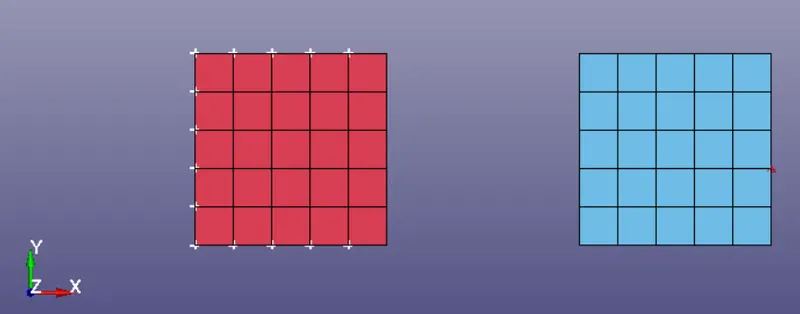

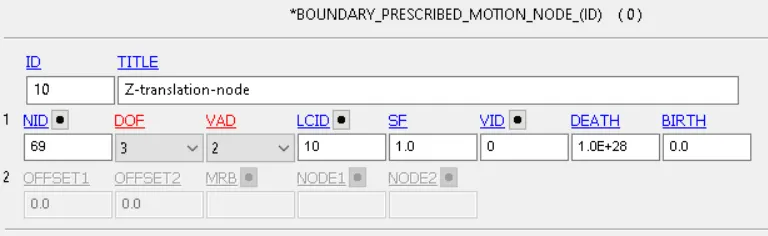
Lastly, we have to use the control termination card and specify our D3PLOT and ASCII file outputs.

Simulation result:

Case 2) Revolute Joint between two deformable bodies

Similar to case 1, we will start by modeling two shell elements with some separation between them using the shape mesher menu. In contrast with the previous case, an elastic material (MAT001) and a section shell keyword card will be created and assigned to both parts

From there, 4 extra nodes have to be created and joined to the shell parts with CNRB elements. It is important to use the newly created nodes as the P-node instead of the center of mass

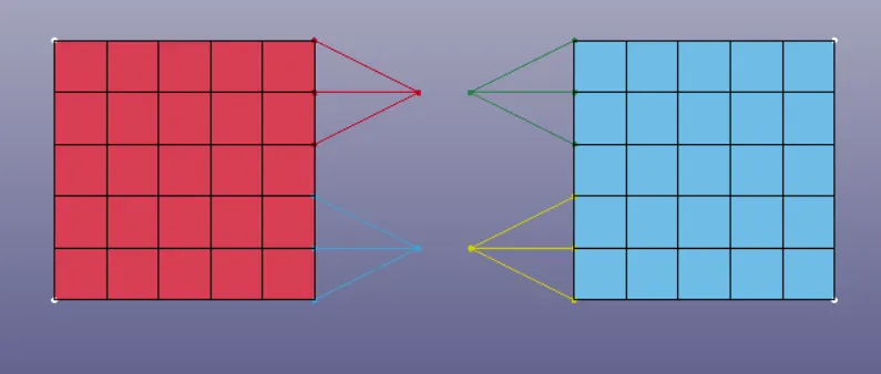
Then, the CNRB elements are translated using the edit node menu to make them coincident

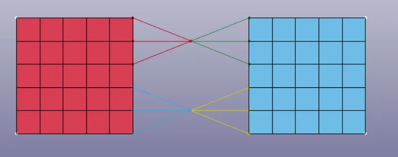
The last step is to define our Constraint Joint Revolute keyword card as well as the same boundary conditions as in case 1)

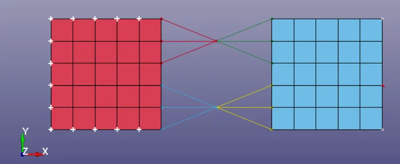
Once again, before running the simulation we must include the control termination card and the ASCII outputs.

Simulation result:

Case 3) Cylindrical Joint between two rigid bodies

The first step is to create two hollow cylinders by using the shape mesher menu

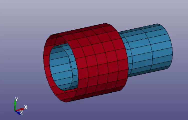
Then, two pair of nodes that are concentric to the cylinder must be created. This will be used to define the axis from which rotation and translation is allowed

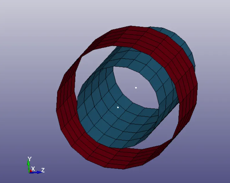
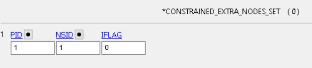
This pair of nodes have to be associated with the cylinders using a constrained extra node set keyword

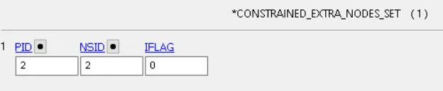
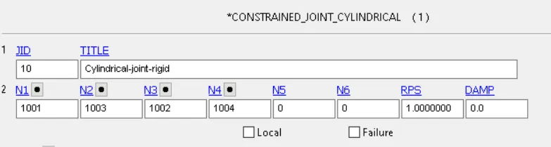
The joint behavior has to be specified using a Constraint Joint Cylindrical Keyword. We must remember that nodes 1 and 3 will belong to the outer cylinder, while nodes 2 and 4 to the inner one.

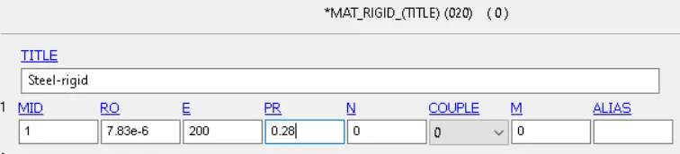
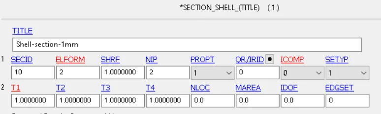
Once everything is defined, we must proceed by assigning a rigid material (MAT020) and a section shell keyword to both parts.

Lastly, some boundary conditions must be stablished to allow for the joint to work properly. In this case we will use:

• All fixed DOF's in the outer cylinder

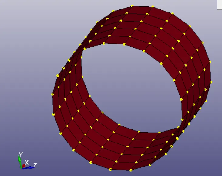
• Initial rotational and translational velocity on the inner cylinder around the X axis

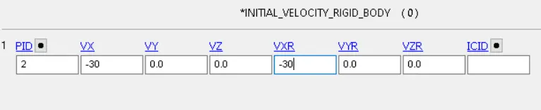
Lastly, a control termination card and D3PLOT/ASCII files must be specified before running the simulation

Simulation Result:

Case 4) Cylindrical Joint between two deformable bodies

Similar to case 3) the first step is to create both cylinders using the shape mesher menu. And put the center nodes to use them as P-nodes to create CNRB elements

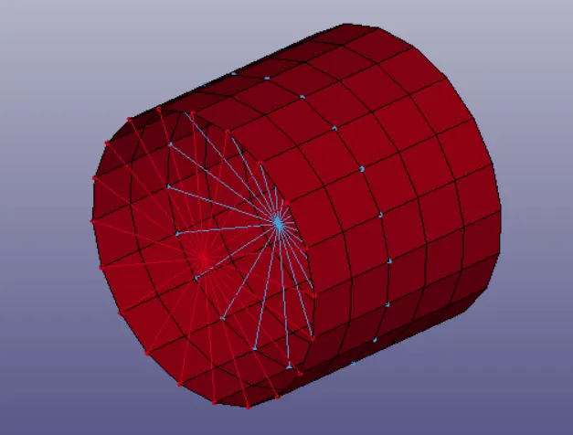
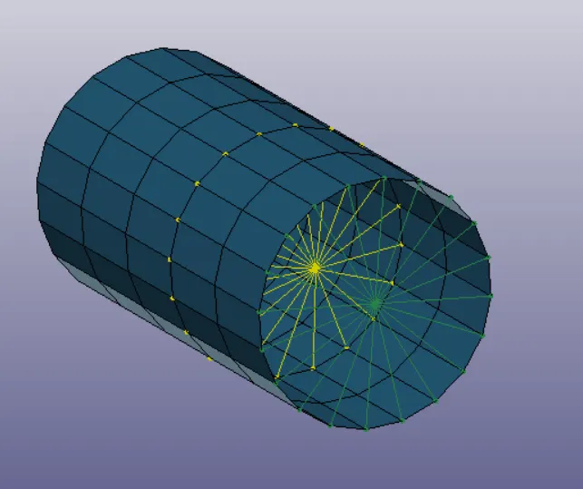
From there, we can create a linear elastic material card (MAT001) and a proper section shell keyword to assign to both parts. Also, we must not forget to use the constrained cylinder joint to define the movement of the parts.

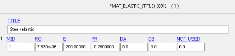
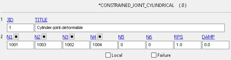
All the other keywords to define the boundary conditions or the output files remain the same as in the previous case

Simulation Results

Case 5) Spherical Joint between two rigid bodies

Similar to the previous cases, the first step is to use the shape mesher menu to create two concentric hollow spheres, and delete the upper elements of the outer part

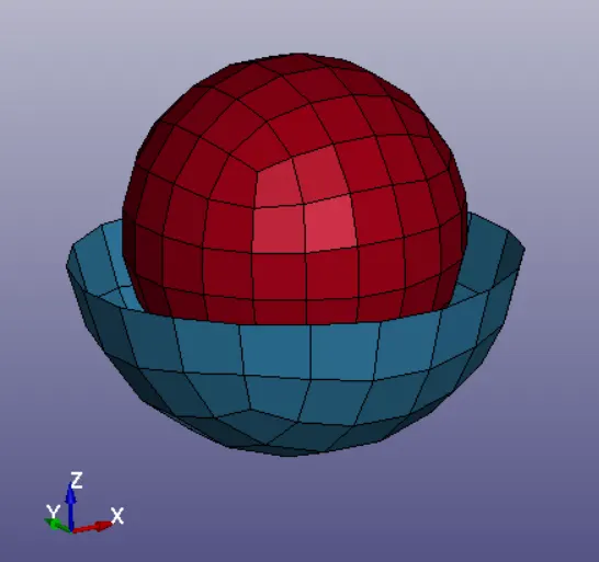
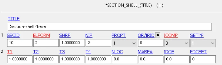
From here, we must create both a rigid material (MAT020) and section shell keyword to assign to both parts

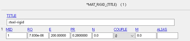
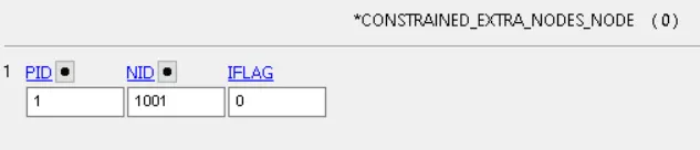
The next step is to create two nodes that are concentric to both spheres and assign them to each part using a Constrained Extra Node keyword

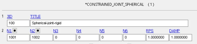
Then, a constrained joint spherical keyword can be used to stablish the joint behavior

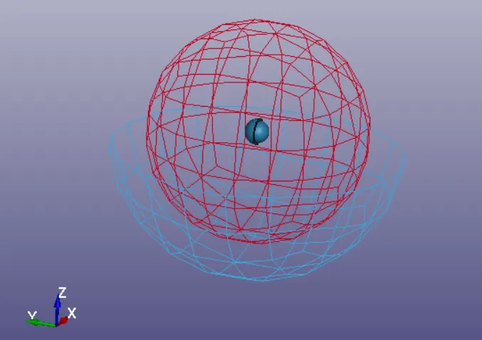
Lastly, some boundary conditions must be applied to the model in order to make the joint work. In this case we will use:

• Fixed all DOF's in the outer sphere

• Any value of rotational speed in all axes in the inner sphere nodes

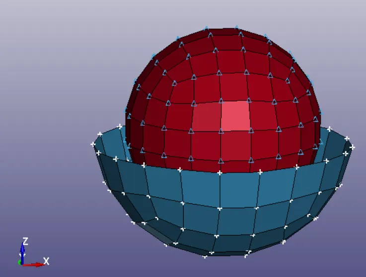
Simulation results:

Case 6) Spherical Joint Between two deformable bodies

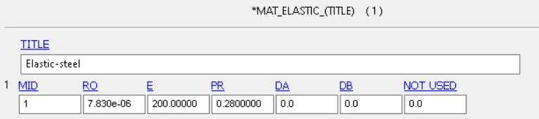
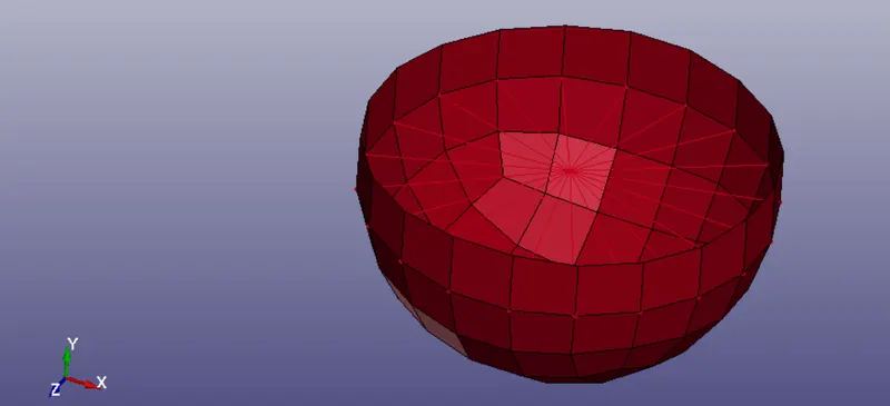
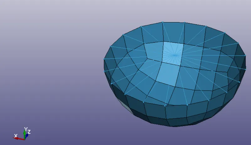
Similarly to previous cases, the only difference between using a rigid or a deformable body is that we have to use a different material keyword (MAT001) and connect our middle nodes through CNRB elements instead of using the Constrained Extra Node Keyword.

Elastic Material Definition:

CNRB Part creation:

From there, the spherical joint is defined using the exact same keyword

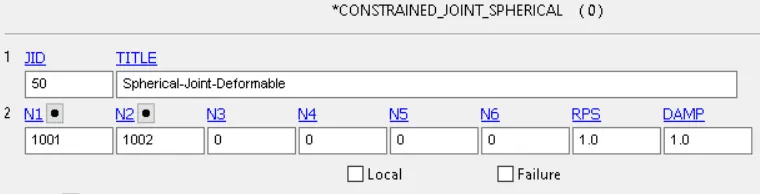
The boundary conditions used for the model include fixed all DOF's in the outer sphere, and initial rotational speed in all axes for the nodes in the inner sphere

Simulation Results:

Case 7) Translational joint between rigid bodies

This final case is similar to the cylindrical joint, yet, the translational joint differs in the sense that the geometry doesn't allow for rotation along the axis. Thus, we will first start by creating two hollow boxes using the shape mesher menu

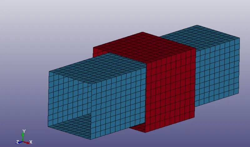
The next step is to create three pairs of coincident nodes. Two pairs have to aligned so that they can define the axis of translation, and the last pair must have a slight offset so that it can prevent rotation in the other axes

These nodes must be associated with their respective parts using a constrained extra node keyword

The joint behavior is defined using a constrained joint translational keyword

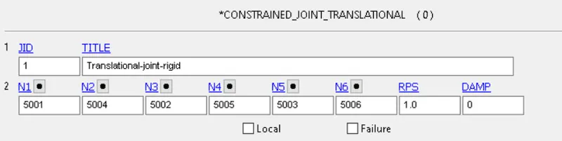
From there, a rigid material (MAT020) and a section shell keyword card with 1mm thickness are created and assigned to both parts, as shown in all previous cases.

Lastly, some boundary conditions are required to properly simulate the behavior of the joint. In this case, we will use:

• All DOF's fixed on the outer box

• Initial translational speed of 50mm/s in the Z axis on the inner box

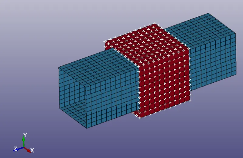
From there, all of the remaining keywords regarding control termination outputs and ASCII files remain the same

Simulation Results

Case 8) Translational Joint between two deformable bodies

The major difference between this case and the previous one is that instead of integrating the extra nodes to both parts with a constrained keyword, we must use CNRB elements, as shown in the following pictures

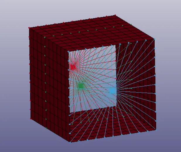
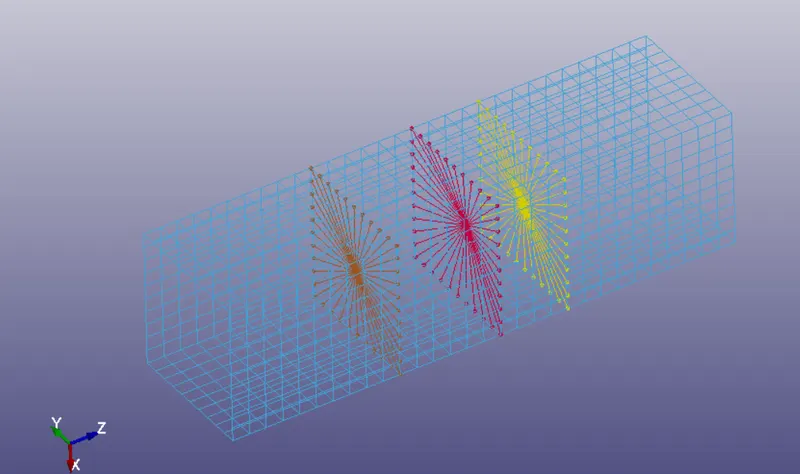
Another important difference is that we have to use a different material keyword, in this case, we will use an elastic material definition (MAT001)

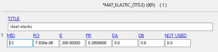
The rest of the keywords remain exactly the same as the previous case.

Simulation result: