Week 11: FSAE Car Project

FSAE CAR PROJECT

Aim:-

To simulate the FSAE car model with a lot of turns and straight track conditions with 45kmph and 75kmph of lap speed.

Objective:-

Phase 1:-

Run a Virtual tunnel no-hydro test and a coarse simulation test to prove that the simulation runs. The Virtual wind tunnel boundary conditions and physical models can be assumed.

Phase 2:-

Race-1

• Race track conditions - Lots of Turns
• Average lap speeds - 45kmph
• 70% turns at 45 degree
• 20% turns at 80 degree
• 10% turns at 20 degree

Race-2

• Race track conditions - Straight
• Average lap speeds - 75kmph

SIMULATION PROCESS:-

A. Geometry:-

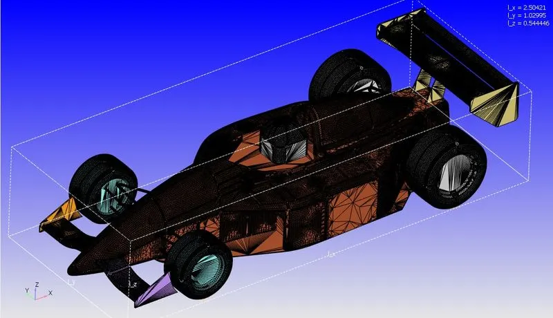
• The STL geometry was imported from inches to meters.
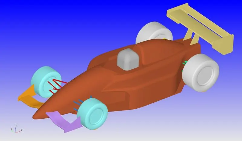
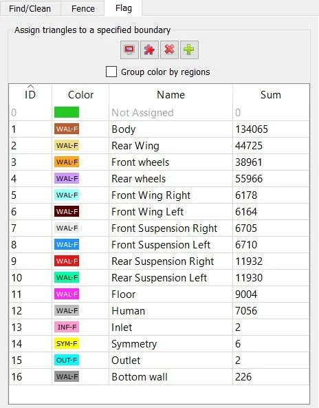
• In the geometry, all the error is cleanup and the front wing, rear wing, tyres, suspension links are flagged as a separate boundary condition.
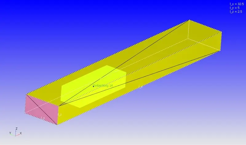
• The virtual wind tunnel is created with appropriate dimensions.
• The bottom wall of a wind tunnel is merged with the flat surface of the tyre in the lower end section.

Boundary Flagging:-

B. Case Setup:-

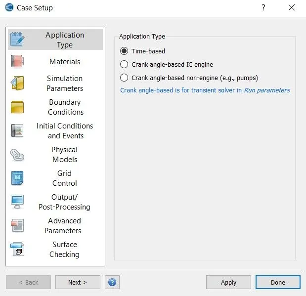
1. Application Type:-

2. Material:-

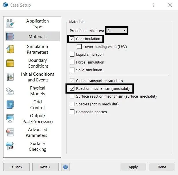
• Gas simulation - Redlich-Kwong
• Global transport parameters
• Reaction mechanism - O2 & N2

3. Simulation Parameters:-

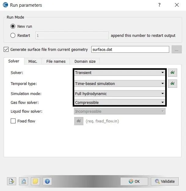
• Run parameters
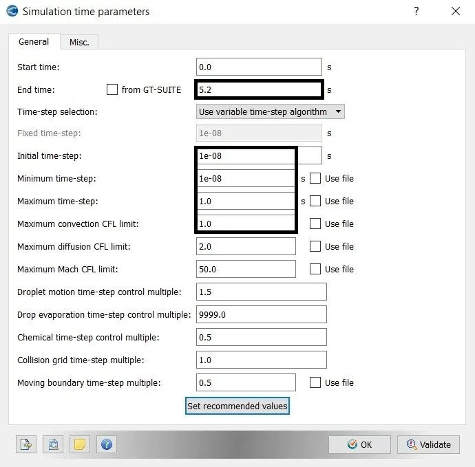
• Simulation time parameters
• solver parameters

End time = 2 x (Total length/velocity)

= 2 x (32.5/12) = 5.2 seconds

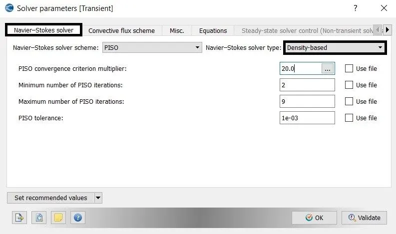
4. Initial conditions and Events:-

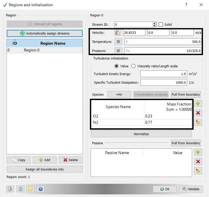
5. Boundary conditions:-

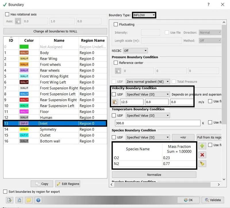
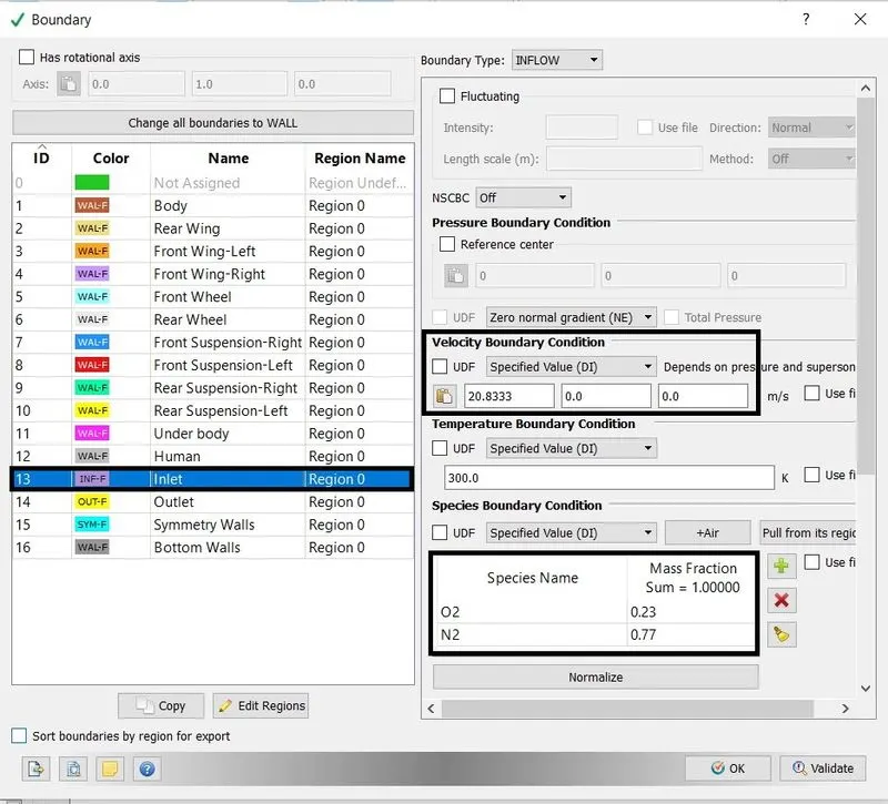
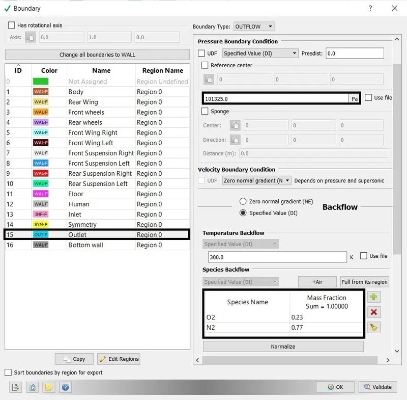
• Inlet - Inflow with 12.5m/s and 20.8333m/s
• Outlet - Outflow
• Symmetry - Symmetry conditions
• Bottom wall - Law of wall
• Body - Law of wall
• Rear wing - Law of wall
• Front wing right - Law of wall
• Front wing left - Law of wall
• Front suspension right - Law of wall
• Front suspension left - Law of wall
• Rear suspension right - Law of wall
• Rear suspension left - Law of wall
• Underbody - Law of wall
• Human - Law of wall

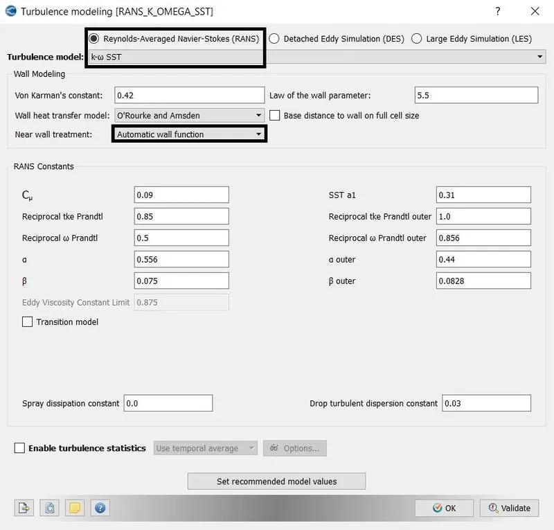
6. Physical Model:-

7. Grid Controls:-

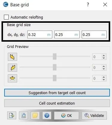
• Base Grid
• Fixed Embedding

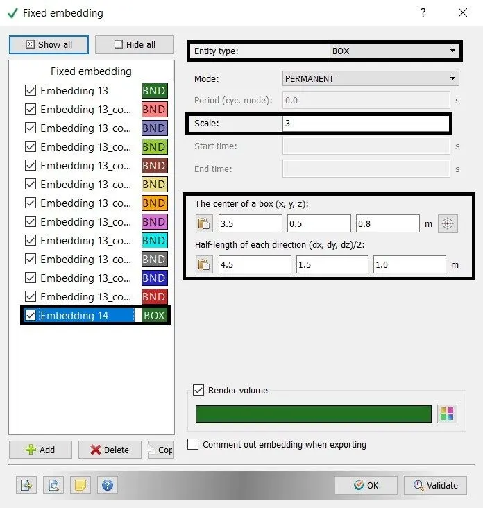
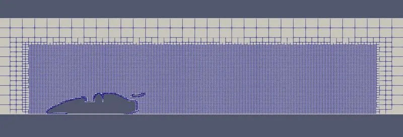
Embedding for all boundaries of a car with a scale value of 3 and layer 1.

8. Output/Post-Processing:-

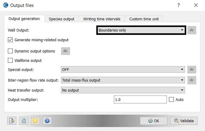
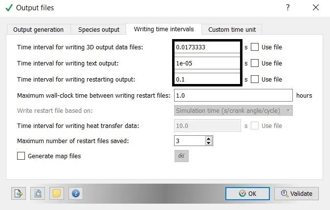
C. Execute the Simulation:-

• The Executable file "mpiexec.exe" and "converge.exe" is pasted in the input files.
• To run the simulation in Cygwin by using the command

mpiexec.exe -n 2 converge.exe restricted </dev/null> logfile &

• After the simulation is complete, the output files can be converted into Paraview VTK in-line binary format to post-process the result in ParaView.

mpiexec.exe -n 2 post_convert_30_msmpi.exe

D. Post-Processing the Result:-

Mesh:-

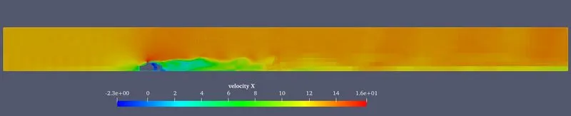
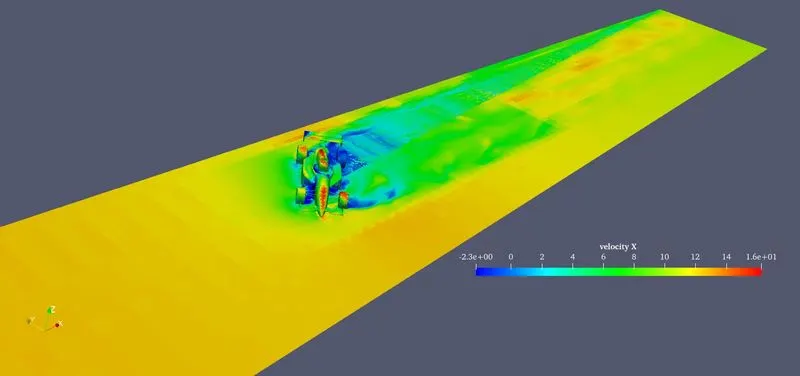
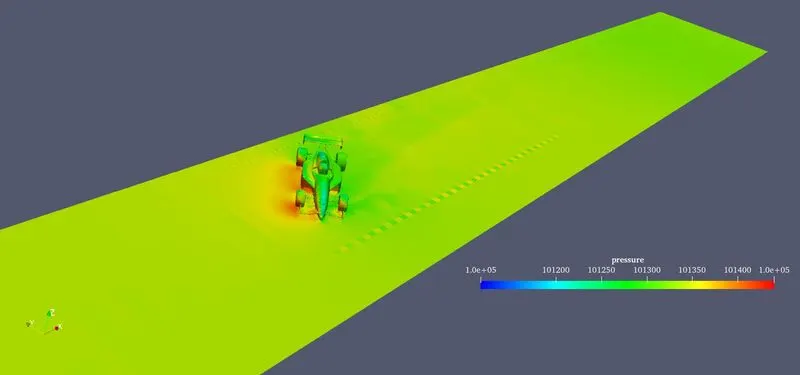
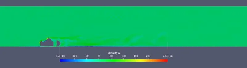
Race -1 [Lot of turns]:-

1. Velocity contour:-

2. Pressure contour:-

3. Vortices:-

4. Total cell count:-

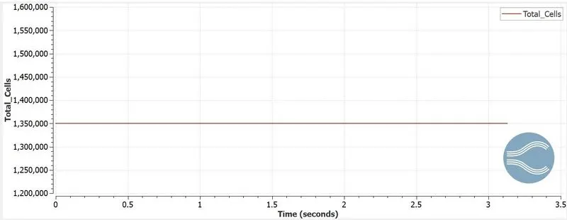
Cell Count = 1350415

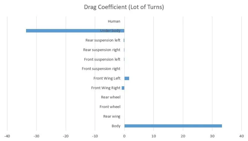
5. Drag Coefficient:-

6. Lift Coefficient:-

7. Animation:-

Race -2 [Straight tracks]:-

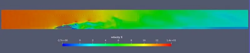
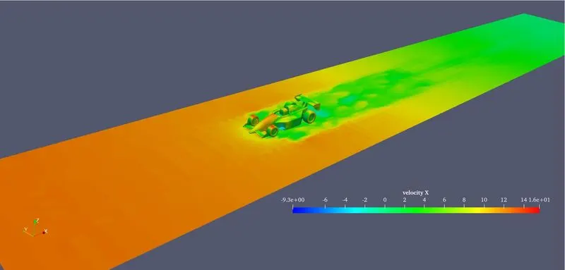
1. velocity contour:-

2. Pressure contour:-

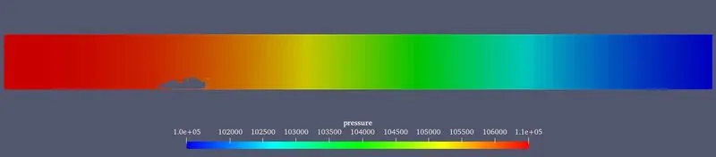
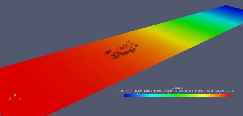
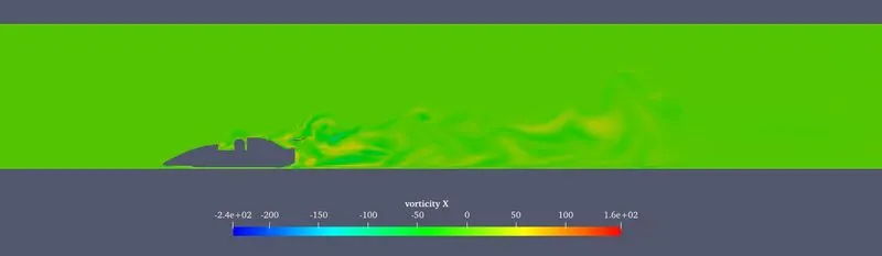
3. Vortices:-

4. Total Cell counts:-

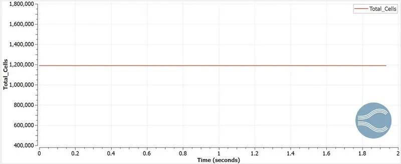
Cell count = 1188514

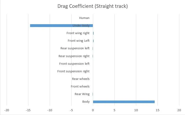
5. Drag Coefficient:-

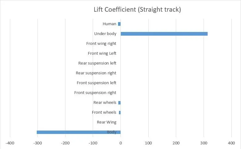
6. Lift Coefficient:-

7. Animation:-

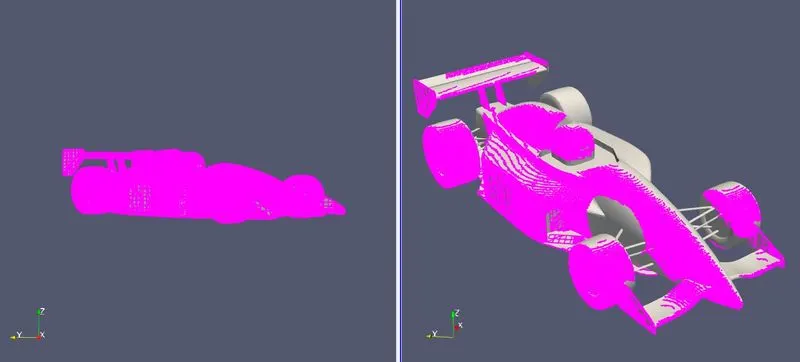
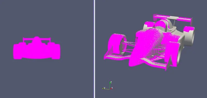
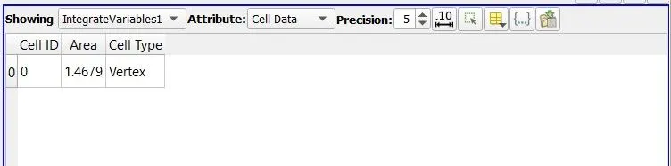
Frontal area calculation:-

The are is calculated from the paraview.

1. Lot of turns track:-

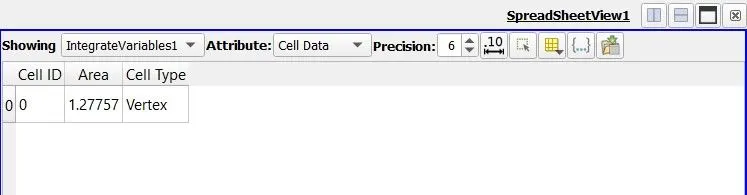
2. Straight track:-

Drag Coefficient and Lift coefficient Calculation:-

Formula :-

• `color(red)("Drag coefficient" = (F_D)/((rho.A.v^2)/(2))`
• `color(red)("Lift Coefficient" = (F_L)/((rho.A.v^2)/(2))`

where,

`F_D = "Drag force 'N'"`

`F_L = "Lift Force 'N'"`

`rho = 1.1761 (kg)/m^3`

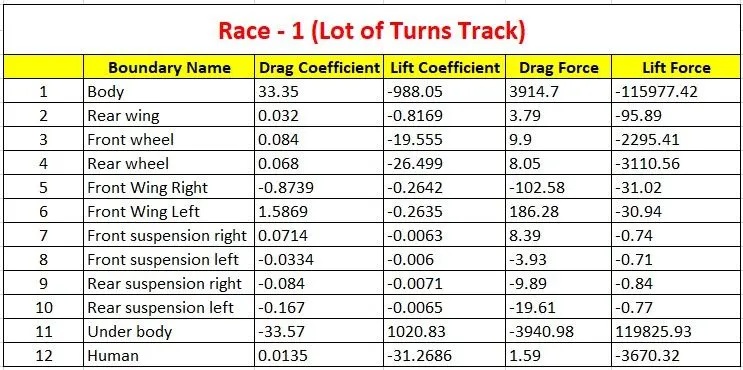
1. Lot of turns track:-

`"Frontal Area" (A) = 1.2775 m^2`

`"Velocity" = 12.5 m//s`

`(rho.A.v^2)/(2) => (1.1761 xx1.2775 xx(12.5)^2)/(2)`

`color(blue)((rho.A.v^2)/(2) = 117.38 N)`

`"Drag coefficient" = (3914.70)/(117.38) => color(blue)(33.35)`

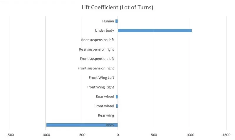
`"Lift coefficient" = (-115977.42)/(117.38) => color(blue)(-988.05)`

2. Straight Track:-

`"Frontal Area" (A) = 1.4679 m^2`

`"Velocity" = 20.8333 m//s`

`(rho.A.v^2)/(2) = (1.1761 xx1.4679 xx(20.8333)^2)/(2)`

`color(blue)((rho.A.v^2)/(2) = 374.64 N)`

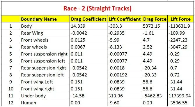
`"Drag coefficient" = (5372.15)/(374.64) => color(blue)(14.339)`

`"Lift coefficient" = (-113631.90)/(374.64) => color(blue)(-303.30)`

E. Conclusion:-

• From the simulation, it can be concluded that the drag coefficient and lift coefficient is high in the race-1 condition because the velocity is low compared to race-2 and a lot of turns reduce the speed of the car.
• Here lift force is z-direction but the values are negative which means the downforce is acting on the car.
• But in both races, the Underbody has a positive value that lift force is acting on the bottom of the car. so the downforce is not acting in the Underbody region.
• The maximum amount of downforce is acting on the body in both cases.
• If we want to increase the downforce the angle of the rear wing should be increased.

Case Setup Link -

1. Race-1 (Straight Track)

2. Race-2 (Lot of Turns)

Excel data for Drag & Lift Coefficient:

Drag and Lift