Week-11 Challenge: Braking

Q1)For a defined driving cycle, calculate the energy required for braking.

Braking is one of the cause of the lost of energy in a vehicle.The amount of energy loss depends on the drive cycle. For a highway drive cycle braking loss is comparatively low as less braking is involved. In urban driving cycle braking losses are considerably high because of continuous braking operation.

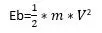
Braking energy is given by,

Where,

m= mass of the vehicle in kg

V=Initial velocity – Final Velocity

Lets calculate braking energy required for UDDS drive cycle.

As UDDS drive cycle time is large let calculate braking energy for initial 150 seconds.

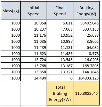
As calculated from the excel sheet the total braking energy required for braking is 116.3 kW.

The excel sheet is attached in the attachements.

Q2)Why electric motor can’t develop braking torque at high speed similar to starting? How electric and mechanical brakes are coordinated?

Regenerative braking allows electric vehicles to use the motor as a generator when the brakes are applied, to pump vehicle energy from the brakes into an energy storage device. Regenerative braking is an effective approach to extend the driving range of an EV.

The regenerative braking torque cannot be made large enough to provide all the required braking torque of the vehicle as it might lead to the deterioration in stability of the vehicle. Also as compared to the torque values of acceleration torque of motor is much higher than decceleration torque.

• At high speed, the motor might be in its constant power region which causes less values of torques produced and this limits the amount of braking torque that is used for regeneration. Hence the peak vlaue of accleration torque and braking torque are not equal.
Electric and Mechanical brakes Co-ordination:

The regenerative braking system may not be used under many conditions, such as with a high State of Charge (SOC) or a high temperature of the battery. In these cases, the mechanical braking system works to cover the required total braking torque.

Thus, cooperation between the mechanical braking system and the regenerative braking system is a main part of the design of the EV braking control strategy and is known as

torque blending.

There are 2 different control strategies for Braking Combinations:

1. Series Control Strategy

2. Parallel Control Strategy

Series Control Strategy:

• A combination of friction-based mechanical braking system with a regenerative braking system that transfers energy to the battery with an integrated control, which distributes the required braking force between the regenerative braking system and the mechanical braking system.
• Series Startegy could give an increase of 15-30% in fuel efficiency and has more consistent braking due to good torque blending capability.

Parallel Control Strategy:

• combination of mechanical and the regenerative braking system, operated simultaneously without an integrated control.
• The regenerative braking force is added to the mechanical braking force which cannot be controlled.
• The regenerative torque is determined by considering the motor capacity, battery SOC, and vehicle velocity. The regenerative braking force is calculated from the brake control unit by comparing the demanded brake torque and the motor torque available.

Application of Braking Combination: EDIB (Electric Driven Intelligent Brake) in NISSAN LEAF

• EDIB allows and controls optimization of the regenerative brake and regular friction brake (hydraulic brake).
• The system produces an adequate braking force keeping energy regeneration increased as much as possible.

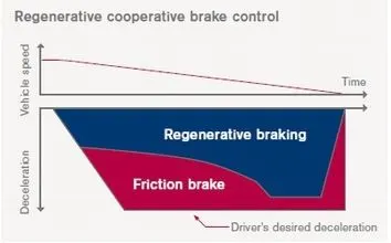
• At higher speeds, a combination of regenerative and friction braking is applied.
• At lower speeds, regenerative braking is given a higher proportion for maximised energy conversion.

Q3)Make a MATLAB program which plots contour of given motor speed, torque and efficiency values. Attach the code as a .m file attach a screenshot of all the plots.

MATLAB Code:

clear all;
clc;
% Speed Array
omega = linspace(0, 300, 100);
% Torque Array
T = linspace(0, 2000, 100);
% Meshgrid
[X,Y] = meshgrid(T, omega);

% Loss Coefficients
cu = 0.17; % Copper coefficient
fe = 0.006; % Iron coefficient
win = 0.000015; % Windage coefficient

% Losses
cu_loss = cu*(Y.^2); % Copper Losses
fe_loss = fe*(X.^2); % Iron Losses
win_loss = win*(X.^3); % Windage Losses
cond_loss = 18; % Conduction Losses

% Output Power
P_out = (X.*Y);
% Input Power
P_in = P_out + (cu_loss) + (fe_loss) + (win_loss) + (cond_loss);
% Efficiency
n = ((P_out)./(P_in));

% Efficiency values for contour
W = linspace(0.75, 0.95, 10);
% Contour Plot
contour(X,Y,n,W)
xlabel('Angular Speed, rad/s')
ylabel('Torque, Nm')
title('Speed, Torque and Efficiency characteristics of Motor')

Explanation:

In this MATLAB script, we create arrays for the speed and the torque of the motor using the ‘linspace’ command. For the speed, consider a range of values from 0 to 2000 radians per second whereas for the torque, consider a range of values from 0 to 300Nm.These arrays are then used to create 2D grid coordinates using the ‘meshgrid’ command. These coordinates will help in the creation of the contour plot. In order to find the efficiency of the motor, we need to consider the various losses that occur in the motor’s operation. These are:

Copper losses

Iron losses

Windage losses

Conduction losses

These various losses are dependent on the speed and the torque of the motor. They each also have a characteristic constant of proportionality which are all assumed for the following calculations and represented as 'K'. In each calculation, the speed and the torque are represented respectively as: ω and T.

Copper losses = KCu⋅ω2

Iron losses =KFe⋅T2

Windage losses =Kw⋅T3

The values of coefficients are taken as general values. Conduction losses are assumed to be 18 Joules.

Finally we plot the contour with the 'contour' command. In addition, an array for the efficiency values we want to plot for is created called 'W' and is assigned for values ranging from an efficiency level of 0.75 to 0.95. This array is used in the creation of the contour. Axis labels and a title is also made for better readability.

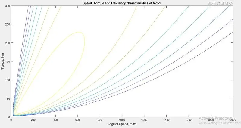
From this contour plot, we can see that the highest level of efficiency arises in the innermost contour plot and this efficiency decreases as the contours increase in size from the innermost contour.