Introduction to HEV using MATLAB and Simulink - Calculation of Braking Energy, Regen Braking Strategies & Plotting E-Motor Efficiency contour map

1. For a defined driving cycle, calculate the energy required for braking.

The braking energy formula is as follows :

`B_(en ergy) = 1/2*m*(v_i^2 - v_f^2)`

Where, `B_(en ergy)`is the braking energy is Joules (J), `m` is the mass in kg , `v_i`is the initial velocity of the vehicle in m/s and `v_f`is the final velocity of the vehicle in m/s.

To convert the energy from Joule(J) to KWh, the value is divided by 3.6 x 10^6.

The UDDS cycle is used for this particular calculation. In this code, first braking scenario has to be identified, and then the formula has to be applied. The braking scenario happens when the velocity is decreases. In the code, first those instances where the velocity decreases is found, and then the braking energy formula is applied, which gives the instantaneous braking energy. All these values are added up to obtain the total energy required for braking in that particular drive cycle.

The matlab code is as follows :

clear all 
close all
clc

load CYC_UDDS.mat
v = 0.44704*cyc_mph(:,2); 
m = 1000; 

i = 1 ;

for i = 1: length(v)-1
if v(i+1) < v(i)
    b(i) = (0.5*m*((v(i))^2 - (v(i+1))^2))/(3600*1000);
    i = i+1 ; 
else
    b(i) = 0;
    i = i+1 ;
end 
end 

Braking_energy = sum(b);

figure(1)
grid on 
plot(v) ; 
xlabel('Time in seconds'); 
ylabel('Velocity in m/s');
title ('Drive Cycle'); 

figure(2)
grid on
plot(b); 
xlabel('Time in seconds'); 
ylabel('Instanteous braking energy in KWh');
title ('Braking Energy'); 

UDDS cycle table : https://drive.google.com/file/d/1yGWCxAoB5YErEmp7a6Qmc4IbMzbtQLAz/view?usp=sharing

The output plot indicates the velocity plot and the instantaneous braking energy across the entire drive cycle.

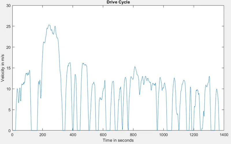
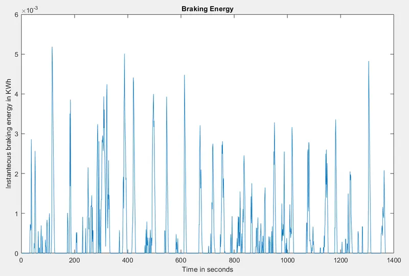
The first plot is the velocity curve (in mph) for an UDDS drive cycle. The second plot indicates the instantaneous braking energy in KWh at every time instant for the given drive cycle, which is calculated using the formula mentioned before. The mass of the vehicle was kept at 1000kg, under these conditions the total braking energy required in the UDDS drive cycle is 0.583 KWh.

2. Why electric motor can’t develop braking torque at high speed similar to starting? How electric and mechanical brakes are coordinated?

The Electric motor torque-speed characteristics is as follows :

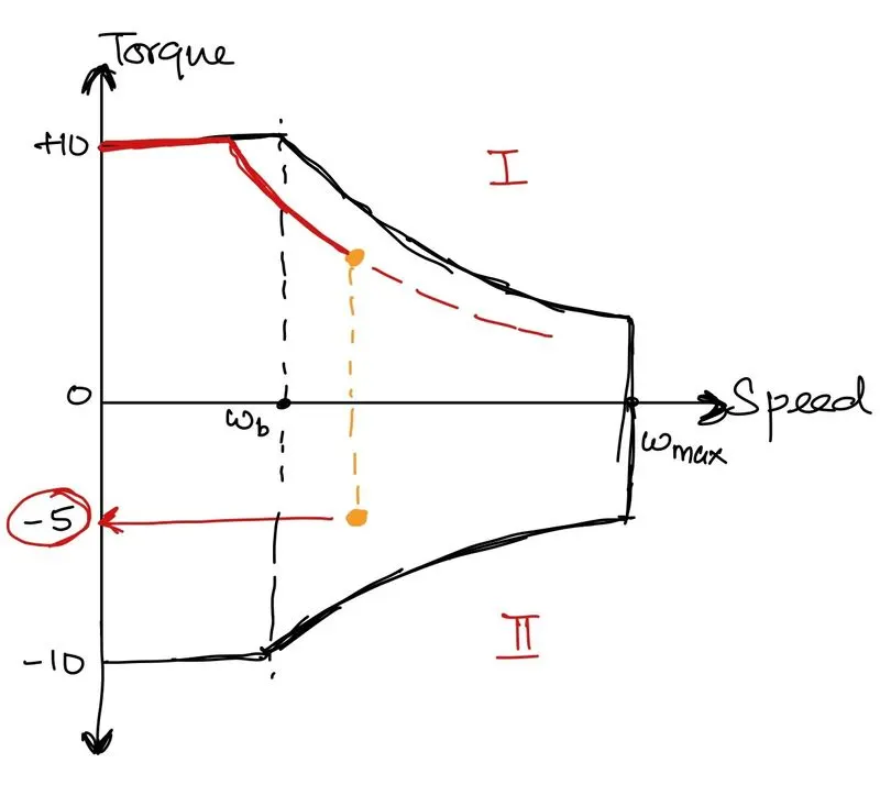
During an acceleration conditions, while starting, the motor starts with high constant torque, say like the 10Nm in the above motor curve until the base speed, and beyond the base speed, the torque starts decreasing, as the operating point enters the constant power region. On the other hand while braking, the motor is operating at a higher speed (more than the base speed), in such cases the peak braking torque is not available for the motor. In the above example curve, it can be observed that when the operating point is transferred from the first quadrant to the second quadrant, the braking torque is -5Nm. As in this case the peak braking torque is always less than the peak accelerating torque.

This affects the amount of energy regenerated during braking. Since peak braking torque is decreased, the amount of energy regernated also decreses. Other reasons for lesser regenerative energy during braking is the lower limit of charging current that can be given to the battery. This type of regeneration of energy is possible only with the help of bi-directional power converters.

The electric and mechanical brakes are coordinated in two different control strategies:

- Series control strategy: In this case, the two braking systems work one after the other. Most commonly, the electric brakes start to operate ahead of the mechanical brakes. The mechanical braking system starts operating only when the electric brakes reaches its maximum limit (max brake torque).

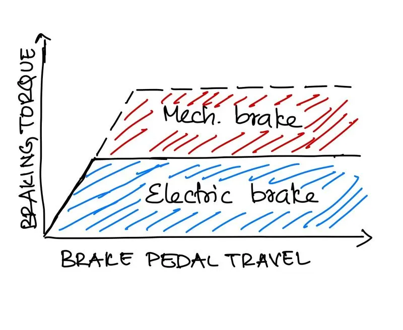
- Parallel control strategy: In this case, both the electric and mechanical braking work simultaneously to provide the desired braking torque.

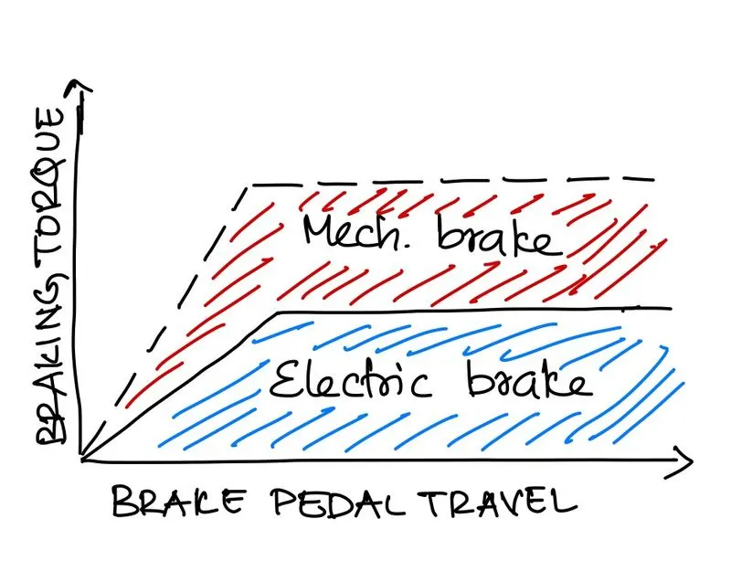
The application of these strategies depends on comfort required and energy recovery required.

3. Make a MATLAB program which plots contour of given motor speed, torque and efficiency values. Attach the code as a .m file attach a screenshot of all the plots.

The efficiency of the motor is given by :

`eta = (O.P)/(I.P)`

Where, `eta`is the efficiency, `I.P` is the input power and `O.P`is the output power.

The relation between the input power and the output power is as follows :

`I.P = O.P + Losses`

The motor generally has the following types of losses :

- Copper losses : These losses occurs at the windings in the stator and the rotor, and it depends on the current flowing through the windings and the internal resistance. Since the current and torque are directly proportional, the copper losses can also be represented in terms of the output torque.

Copper losses = `I^2*R = K_c*T^2`

- Iron Losses : This loss is dependent on the magnetic field, and hence this loss is also called as the magnetic loss. This loss depends on the magnetic flux, and hence also depends on the speed of the motor. The constant `K_i`depends on the magnetic field, due to which it is constant for a PMDC motor.

Iron Losses = `K_i *omega`.

- Windage and Friction losses: These are mechanical losses, caused due to the wind resistance and friction. This is represented by the following equation.

Windage Losses = `K_w*omega^3`

All the other losses are represented using a constant `C`

Hence the total losses in a motor is given by :

Losses = `K_c*T^2 + K_i*omega + K_w*omega^3 +C`

The input power is the electrical power given to the motor, the output power is the mechanical power. This mechanical power is the product of the torque and speed of the motor. These formulas are used to create the matlab code.

The matlab code is as follows :

close all
clear all
clc

t = linspace(1,200);
n = linspace(0,1000); 

[T,N] = meshgrid(t,n);
Out_P = T.*N;

Kc = 0.2;
Ki = 0.008;
Kw = 0.00001; 
C = 20; 

CuL = Kc*(T.^2);
IrL = Ki*N;
WiL = Kw*(N.^3);

In_P = Out_P + CuL + IrL + WiL + C ; 
eff = Out_P./In_P;

eff_cont = [0.7 0.75 0.8 0.85 0.9 0.91 0.92 0.93];

figure(1)
grid on 
plot_line = contour(N,T,eff,eff_cont);
xlabel('Speed in rad/sec');
ylabel ('Torque in Nm');
title( 'Electric Motor Efficiency Plot');
clabel(plot_line);

The electric motor efficiency plot is as follows :

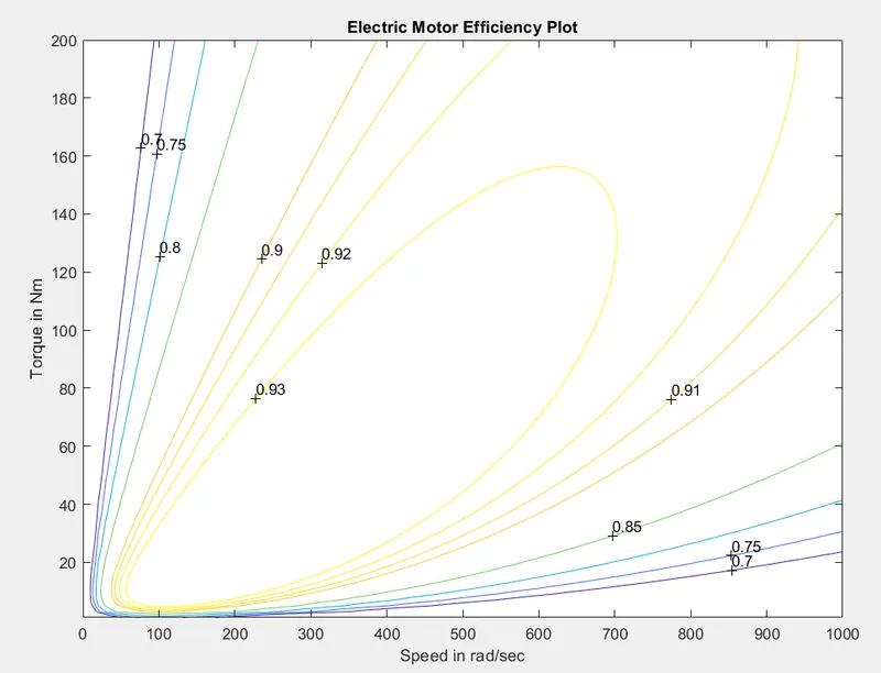
The above plot represents the efficiency contours in the torque-speed plot of the motor. The control strategies are formed such that the motor is operated in the higher efficient region. At these torque-speed operating points the losses indicated above are at their lowest.