Week-11 Challenge: Braking

1. For a defined driving cycle, calculate the energy required for braking.

Approach-

For this question, we consider the UDDS driving cycle. We first compute the energy at each of the driving cycle sample using,

`E = 1/2 mv^2` where,

`m` is the mass of the vehicle and v is the velocity.

Then, the energy difference with the consequent step is computed. I the energy is seen to be depreciated, then this difference is the braking energy consumed. The total braking energy required is the accumulation of these differences.

The approach to find the energy required for braking is implemented in MATLAB as shown below (code attached), assuming the vehicle mass to be 2000kg (ignoring/including moment of inertia effects). The results then follow.

Code-

clear
close all
clc

% Vehicle parameters
m = 2000; %kg

% Download driving cycle
DC = xlsread('UDDS.xls');
t = DC(:,1);
vel_mph = DC(:,2); vel = 0.4470*vel_mph; % convert speed to m/s

% Compute energy lost/gained at each step
energy_t = (1/2)*m*(vel.^2); % Vehicle energy at each step
energy_acceleration = zeros(length(t),1); % Initiallize acceleration array
energy_braking = zeros(length(t),1); % Initiallize braking array
for i = 1:length(t)-1
if energy_t(i) < energy_t(i+1)
energy_acceleration(i) = energy_t(i+1) - energy_t(i);
else
energy_braking(i) = -(energy_t(i+1) - energy_t(i));
end
end

energy_braking_kJ = energy_braking/1e3;
energy_braking_cumulative = cumsum(energy_braking)/1e3; %kJ
energy_braking_total = energy_braking_cumulative(end); % kJ

% Output
figure;
title('Evaluation for UDDS driving cycle')
subplot(3,1,1)
plot(t,vel);
xlabel('t (s)');
ylabel('Velocity (m/s)');
subplot(3,1,2)
plot(t, energy_braking_kJ);
xlabel('t (s)');
ylabel('Braking energy (BE) (kJ)');
subplot(3,1,3)
plot(t, energy_braking_cumulative);
xlabel('t (s)');
ylabel('Cumulative BE(kJ)');

energy_braking_total

Results-

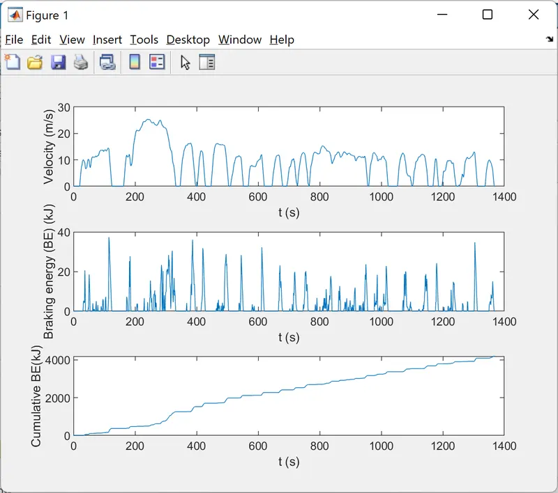
The output of the above code is shown below.

energy_braking_total =

4.1961e+03

We see that the total energy required for braking is approximately 4196.1 kJ.

Note that in this evaluation, we inherently assume a linear (or average) acceleration between time samples. Further, the effects of aerodynamic resistance and rolling resistance are ignored.

2. Why electric motor can’t develop braking torque at high speed similar to starting? How electric and mechanical brakes are coordinated?

Why electric motor can't develop braking torque at high speed-

The figure below shows a general torque-speed relation for a motor,

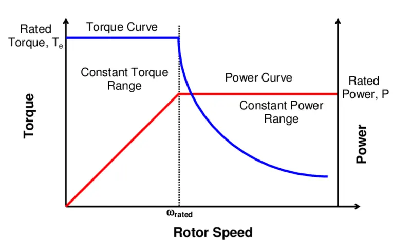
It is seen from this map that, at low speeds, the motor is able to deliver maximum torque to the rotor. This is called the constant torque region. However, at higher speeds, where the motor operates in the constant power region, it is not able to achieve maximum torque. This happens because, here, the rated voltage is exhausted. Consequently, high torque is not developed for braking at high speeds as well. Note that, the torque-speed map for the braking region is (almost) a mirror effect of the above shown characterestic.

How electric and mechanical braking are coordinated-

In mechanical braking, the braking is accomplished by power/energy dissipation through friction by use of for example, hydraulic or disc brakes. Here the braking energy is not re-usable. In electric braking, the braking is brought about by recuperating the braking energy back into the battery by 'reverse current' i.e. allowing regenerative braking which results in more efficient energy usage. However, it may not always be possible to have the full braking required by regenerative method and in these cases, generally, mechanical braking is used in addition (combination). The two braking methods are in general oco-ordinated in two ways as stated below,

i. Series- Only one of the methods is applied at a time, followed by the other, untill the required braking is achieved.

ii. Parallel- Both the methods of braking are applied simultaneously.

The braking strategy is based on a trade-off between comfort and efficiency.

3. Make a MATLAB program which plots contour of given motor speed, torque and efficiency values. Attach the code as a .m file attach a screenshot of all the plots.

The main losses in an electric motor is due to-
i. Copper losses
ii. Iron losses
iii. Windage losses.
We will try to illustrate these losses and it's impact on motor efficiency using a map.

The required example for an efficiency map of a motor is generated using the MATLAB code shown below,

clear
close all
clc

% Motor loss constants
Kc = 0.2; % Copper loss coefficient
Ki = 0.008; % Iron loss coefficient
Kw = 0.00001; % Windage loss coefficient
C = 20; % Constant loss

% Make axes of motor torque and andgular speed values
T = linspace(1,250, 100); T_mesh = transpose(repmat(T, [100, 1])); % torque values
O = linspace(1,1000, 100); O_mesh = repmat(O, [100, 1]); % angular speed values

% Compute efficiency
Energy_lost = Kc*(T_mesh.^2) + Ki*O_mesh...
+ Kw*(O_mesh.^3) + C*ones(size(O_mesh));
Energy_delivered = T_mesh.*O_mesh;
Energy_total = Energy_delivered + Energy_lost;
Eta = Energy_delivered./Energy_total; % Efficiency map

% Output result
steps = [0.7,0.8,0.9,0.91,0.92,0.925,0.93, 0.95];
O_rpm = O*(30/pi);
contour(O_rpm,T,Eta,steps, 'ShowText', 'On');
xlabel('Motor speed (rpm)');
ylabel('Motor torque (Nm)');
title('Efficiency map for a motor (x100 %)');
contourcbar;

Result-

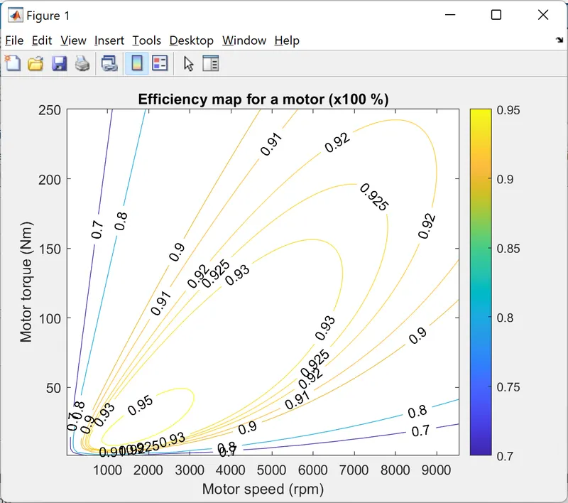
The resulting efficiciency map is shown below,