Week-11 Challenge: Braking

1. For a defined driving cycle, calculate the energy required for braking.

• UDDS (Urban Dynamometer Driving Schedule) is considered
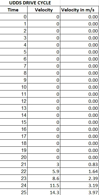
• The driving cycle is saved in excel
• The driving cycle data is imported to workspace
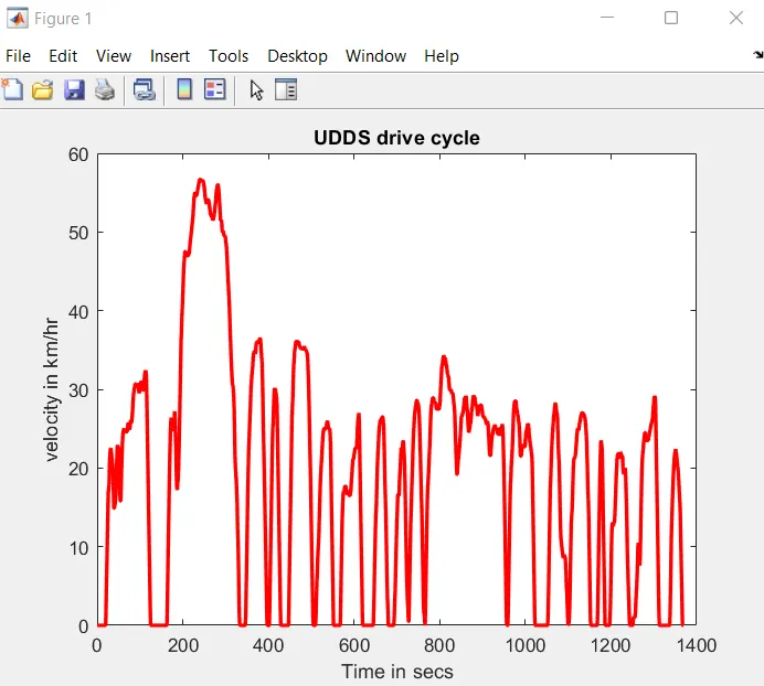
• Matlab script file is written to calculate the energy required for braking and for plotting the drive cycle.

>> edit braking_driving_cycle

braking_driving_cycle.m

% To calculate the energy required for braking in UDDS drive cycle (Urban
% Dynamometer Driving Schedule)
mass = 1000; 
time = Drivecycle(:,1);
velocity_kmph = Drivecycle(:,2);
velocity = Drivecycle(:,3);
n = length(Drivecycle);
for i = 1:n-1
    if velocity(i)>velocity(i+1)
    braking_energy(i) = (0.5)*mass*(velocity(i)-velocity(i+1))^2;
    end
end
braking_energy_total = sum(braking_energy)/1000;
plot(time,velocity_kmph,'r','LineWidth',2);
title('UDDS drive cycle');
xlabel('Time in secs');
ylabel('velocity in km/hr');
fprintf('The total braking energy for given UDDS drive cycle in kJ is %d',braking_energy_total);

>> braking_driving_cycle
The total braking energy for given UDDS drive cycle in kJ is 5.527315e+01

2. Why electric motor can’t develop braking torque at high speed similar to starting? How electric and mechanical brakes are coordinated?

The speed torque characteristics of an induction motor is as shown below:

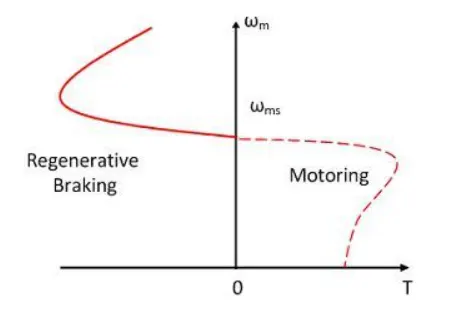
At starting, speed of the motor is zero, hence there is no back emf in opposing the applied voltage. So starting current is more which result in better torque at starting.

In case of induction motor, regenerative braking occurs at a speed greater than the base speed. For speeds greater than the base speed, the motor enters in to constant power mode or field weakening mode. Since it is field weakening mode, the value of torque produced is compromised.

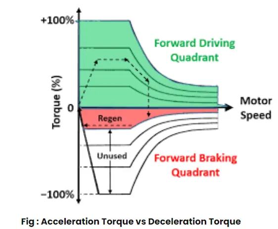
The constant torque and power region are explained in the graph below:

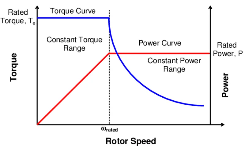
From the graph it is clear that, for speeds above rated speed, motor enters in toconstant power region and the value of torque is compromised.

Regenerative braking can't happen so effectively that we can have all the power to the battery due to limitations of motor, battery and bidirectional power converter. Hence brake control strategies are employed where combined regenerative and mechanical braking is applied.

Main brake control strategies are:

• Series brake control: where mechanical brakes and regenerative brakes are applied one after the other
• Parallel brake control: where mechanical brakes and regenerative brakes are applied simultaneously.

A more effective system introduced recently by Nissan is Electric Driven Intelligent Brake (EDIB). It is basically a parallel brake control system in which mechanical and regenerative brakes are applied simultaneously. They are co-ordinated in such a manner that at low speed percentage of regenerative braking is higher and at high speed both are combined.

3. Make a MATLAB program which plots contour of given motor speed, torque and efficiency values. Attach the code as a .m file attach a screenshot of all the plots.

The main losses in a PMDC motor are:

Copper losses ----> (I^2) R losses = Kc * (T^2)

Iron losses ----> Ki * W

Windage losses ----> Kw * (W^3)

Constant losses ----> C

Total losses = Kc * (T^2) + Ki * W + Kw * (W^3) + C

Input power = Output power + Losses

Efficiency = Output power/ Input power

Efficiency in % = (Output power/ Input power)*100

All mototrs can be mathematically modelled as per the above equation of losses

A matlab script file is written to plot the efficiency contours of electric motors

>>edit contour_plot

contour_plot.m

% Matlab program for plotting efficiency contours of electric motors
% x axis corresponds to motor speed
% y axis correspond to Torque
% First set up arrays for speed range
x = linspace(1,1000);% speed in rad/sec
y = linspace(1,250);
% Allocate motor constants
Kc = 0.2;% for copper losses
Ki = 0.008; % For iron losses
Kw = 0.00001; % For windage losses
ConL = 20;% Constant loss
% Now make mesh
[X,Y] = meshgrid(x,y);
outputpower = (X.*Y);% Power = Torque * speed
B = (Y.^2)*Kc; % Copper loss
C =(X*Ki); % Iron Loss
D = (X.^3)*Kw;% Windage loss
inputpower = outputpower + B + C + D + ConL;
Z=outputpower./inputpower;
%We now set the efficiencies for which a contour is plotted
V = [0.70,0.80,0.85,0.90,0.91,0.92,0.925,0.93];
box off
grid off
contour(X,Y,Z,V);
title('Efficiency contours for Electric Motors');
xlabel('Speed in rad/sec');
ylabel('Torque in N-m');
hold on
%Now plot a contour of the power output
%The array output powers has already been calculated.
%We draw contours at 8kW and 10kW
V = [8000,10000];
contour(X,Y,outputpower,V);

Efficiency contour plots for electric motors are as shown below:

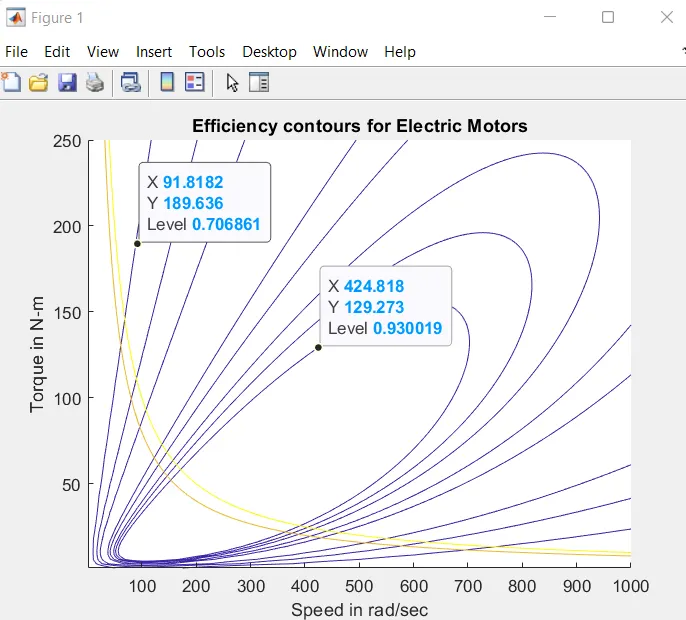
The inner contour corresponds to points of high values of efficiency (more height/level). As it comes outwards, efficiency decreases (height/level decreases). The coordinates of inner and outer contour are marked. From this, it is verified that inner contour has more efficiency than outer contour.