Week-11 Challenge: Braking

1. Energy Required for braking.

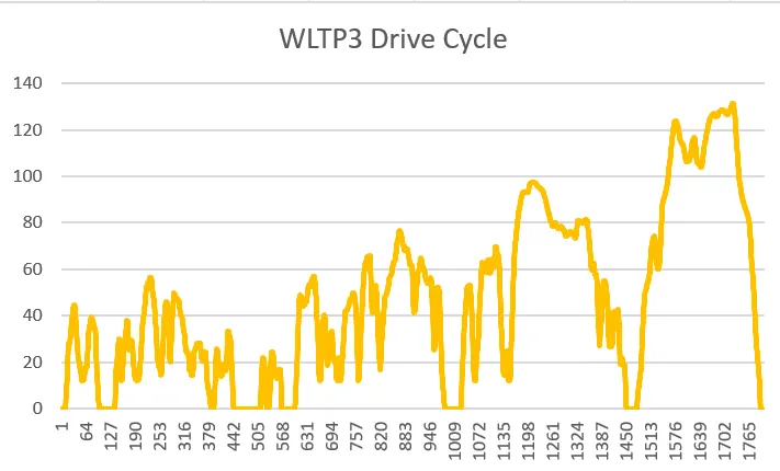
The defined drive cycle taken for consideration is WLTP3 - World Harmonised Light Vehicles Test Procedure - Class 3.

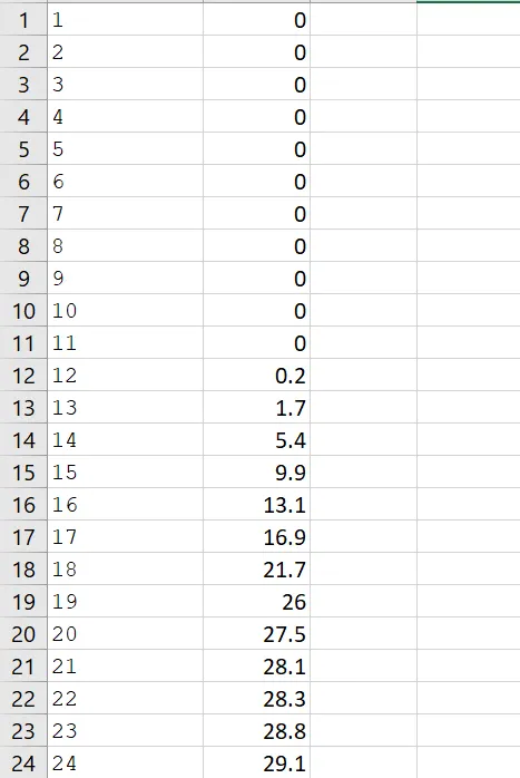
The excel sheet is attached with this document.

The plot of WLTP3 Drive cycle is given below

Calculating the braking energy for Mass M = 500kg , Vf - final velocity after braking , Vi - Initial velocity before braking.

Braking Energy = 1/2 * M * (Vf - Vi )^2

Calculating all the deceleration energies with the above formula, The total braking energy is the sum of all individual energies which is equal to 1187.62 kJ.

2. Speed torque characteristics is shown in the figure below

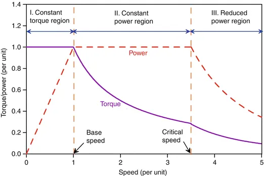
The motor reached the base or critical speed in the constant torque region. Once this critical speed is reached the torque declines in the constant power region. This denotes the acceleration operation of the motor. For deceleration or braking operation the graph is mirrored down which has positive speed and negative torque.

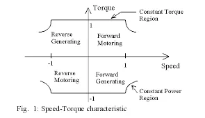
At high speed after acceleration, the vehicle will have reached constant power region and torque would have declined completely. At this point after the application of brakes, the motor will still be in a constant power region. This is because we will be operating at the field tweaking region above the base speed. Thus peak acceleration torque is greater than the peak deceleration torque. Therefore, for acceleration the starting torque is high and for deceleration, torque is low at high speeds.

Electrical and Mechanical Brakes Coordination:

There are three control strategies :

1. Series Coordination: Here either mechanical brakes or electrical regenerative braking is applied.

2. Parallel Coordination: Here both mechanical brakes and electrical regenerative brakes are applied simultaneously.

3. Electric Driven Intelligent Brake:

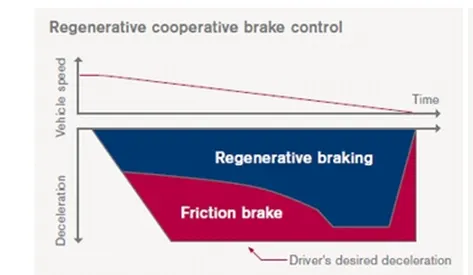
The brakes are made intelligent with the help of an ECU. At low speeds - Regenerative brakes are applied and at high speeds- both regenerative and hydraulic brakes are applied.

3. Contour Plots of given motor speed, torque, and efficiency values.

clear all
close all
clc

speed= linspace(0,1000);
torque= linspace(0,500);

kc= 0.2;
ki=0.006;
kw=0.000010;
k=20;

[x,y] = meshgrid(speed,torque);
copper_loss= (y.^2)*kc;
iron_loss= x*ki;
windage_loss= (x.^3)*kw;

output_power= x.*y;
input_power= (copper_loss+iron_loss+windage_loss+output_power+k);
efficiency=(output_power./input_power);

n=linspace(0.7,0.95,10);
contourf(x,y,efficiency,n);
title('speed-torque efficiency')
xlabel('speed (rad/s)');
ylabel('torque (Nm)');
colorbar
 

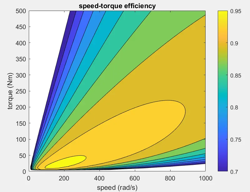
The code has two inputs speed and torque is assigned with the help of linspace command. The motor constants kc,kw, ki, and k are assigned with particular values. The copper loss, iron loss, and windage losses are calculated. The output power is calculated as the product of speed and torque. The input power is output power plus the total losses. Finally, the efficiency is calculated as the ratio of output by the input power. This efficiency is plotted with a contourf function to get a contour plot. It is as shown in the figure below.