Week-11 Challenge: Braking
Aim- Week-11 Challenge: Braking
Main Objective-
- For a defined driving cycle, calculate the energy required for braking.
- Why electric motor can’t develop braking torque at high speed similar to starting? How electric and mechanical brakes are coordinated?
- Make a MATLAB program which plots contour of given motor speed, torque and efficiency values. Attach the code as a .m file attach a screenshot of all the plots.
1. For a defined driving cycle, calculate the energy required for braking.
Drive Cycle- A Drive cycle is the series of data or data points representing the speed of the vehicle versus time. Drive cycles for the vehicle are produced by different countries and organisation to assess the perfromance of the vehicle in varios ways including fuel consumption, milage and pollutant emission. Fuel consumption and emission tests are performed on chassis dynamometers. Tailpipe emissions are collected and measured to indicate the performance of the vehicle.
Another use for driving cycles is in vehicle simulations. More specifically, they are used in propulsion system simulations to predict performance of internal combustion engines, transmissions, electric drive systems, batteries, fuel cell systems, and similar components.Some driving cycles are derived theoretically, as it is preferred in the European Union, whereas others are direct measurements of a driving pattern deemed representative. The most common driving cycles are probably the WLTC, NEDC, SORDS and the FTP-75, the later corresponding to urban driving conditions solely. Driving cycle design is the core technology for these standard cycles.
For this calculation European Urban Dynamometer Driving Schedule or UDDS is used. Here for total braking energy required for the UDDS drive cycle is calculated.
UDDS Drive Cycle- UDDS or FTP-72 The FTP cycle (for Federal Test Procedure) has been created by US EPA (Environmental Protection Agency) to represent a commuting cycle with urban driving including frequent stops. UDDS stands for Urban Dynamometer Driving Schedule, and refers to a mandated dynamometer test on fuel economy that represents city driving conditions which is used for light duty vehicle testing.
It is also known as U.S. FTP-72 (Federal Test Procedure) cycle, LA-4 cycle, in Sweden as A10 or CVS (Constant Volume Sampler) cycle and in Australia as the ADR 27 (Australian Design Rules) cycle.
Though it was originally created as a reference point for fossil fueled vehicles, it is also used to give estimates on how many miles an electric vehicle will travel on a single charge.Urban Dynamometer Driving Schedule (UDDS) driving cycle is a typical urban driving cycle with average speed of 31.51km/h and has frequent braking and acceleration.
Here, the speed values are converted from mph to m/s by the mean of matlab code to have an easy calculation with respect to the metric system.
Braking- Braking is the process of retarding or deaccelerating the speed of the moving vehicle or bring it to rest in the shotest possible distance in less time whenever required. Brakes are the mechanical devices for increasing the frictional resistance that retards the turning motion of the vehicle wheel. It absorbs kinetic energy of the vehicle while in action and this absorbed kinetic energy is rejected out in the form of heat.
The Kinetic energy(E) of the vehicle is given by the equation `E=1/2mv^2`
where m is the mass of the vehicle and v is the velocity of the vehicle at start of the braking.
If the vehicle speed decreases from initial velocity (Vi) to final velocity (Vf), then the required braking energy is given by the formula,
`Eb=1/2m(Vi^2-Vf^2)`
The vehicle mass is assumed to be the actual gross vehicle mass in addition with the 5% of the same for the moment of inertia of all rotating parts in the vehicle. Eg- if the vehicle mass is 2000 Kg then 5% of the 2000 Kg is added to itself, that will become 2100Kg.
The link for the UDDS drive cycle data excel sheet is given below:
The following matlab script is made to calculate the total braking energy required for the UDDS drive cycle:
clc
clear all
close all

mass=input("Enter the Mass of the vehicle:- ");
drive_cycle=xlsread('UDDS_DriveCycle.xlsx');
time=drive_cycle(:,1);
speed=drive_cycle(:,2);
for i=1:(length(speed)-1)
    if speed(i)>speed(i+1)
        br(i)=0.5*mass*(speed(i)-speed(i-1))^2;
    end
end
fprintf("Total brake energy is %d kJ",sum(br)/1000);
subplot(2,1,1);
plot(time,speed);
ylabel("speed(mph)");
title("Urban Dynamometer Drive Schedule drive cycle data");
hold on;
subplot(2,1,2);
plot(br);
xlabel("time(sec)")
ylabel("Brake energy(Wh)");
title("Braking Energy data for the UDDS drive cycle");
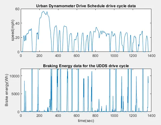
Output- The braking energy is displayed on the command window and the Braking energy plot is given below for the UDDS Drive cycle.

___________________________________________________________________________________________________
2. Why electric motor can’t develop braking torque at high speed similar to starting? How electric and mechanical brakes are coordinated?
Electric motor have high torque producing capability at low starting torque. But as the speed increases the torque values decreases rapidly. At the time of accelerating the vehicle at starting, the maximum torque is available for the motor and is operating at constant torque region. During that period of time the maximum torque is available with minimum speed. But as the motor starts deaccelerating motor characteristic are shifted towards braking region. In this region we don't have much torque available for braking as the motor is running in much high speed.
- During the starting stage, the speed value is very low and the torque produced is very high.
- In the braking stage, the speed of the motor is very high, sometimes greater that its synchronous speed, thus due to high speed the braking torque generated will be very low.
Electric motor have high torque producing capability at low starting torque. But as the speed increases the torque values decreases rapidly
Due to this during braking, electric motor cant develop braking torque at high speed.
Coordination of electric and mechanical brakes
Generally electric motor don't have high torque capacity to handle all the vehicle braking. Hence during the initial braking time, mechanical brakes are used in larger proporting as compared to the electric or regenerative braking so as to slow down or bring the vehicle to complete stop. The mechanical brakes are mostly preferred when the vehicle is moving in somewhat high speed so that the vehicle can slow down or bring to zero speed whenever necessary with minimum possible distance or in minimum possible time.
In an electric Motor, the Total Brake distribution is in two aspects which are Electrical Brake which is called Regenerative Brake, and Mechanical Brake or Classical Brake with a hydraulic cylindrical system. Brake Force distribution must be uniform, If the Regenerative braking power requirement is more than the charging limit of the battery or more than the regenerative capacity of the machine we must apply Mechanical brakes as well. In a practical case, the combination of these two is applied. So usually it is a combined response of Mechanical brake and Regenerative brake. The reason for how this braking force is combined, that particular phenomena are called Brake Control Strategies. There are two Brake Control Strategies, which are Series - In case of Series, we apply Mechanical brake and Regenerative electric brake one after another. We can apply only one brake strategy at a time either apply Regeneratively or apply Mechanical brake. The Series Brake Control Strategy has a further classification, that is based on whether we want the comfort of driver or Brake behavior compared to energy efficiency. Parallel - In the case of Parallel, we apply both brakes simultaneously. This Particular Parallel braking is going to happen both at a time. Electric Driven Intelligent Brake (EDIB) is a combination of Hydraulic brake or Mechanical brake along with a Regenerative brake. It is a Parallel braking technique. The Control criteria such that at low speed use regenerative braking higher and at high speed or during the initial braking period we actually combine the both.
Once the braking torque value starts to decrease, the regenerative braking is increased in proportion. Basically there are two different brake control strategies one is series and the second is the parallel
1. Series brake control
- Series braking with optimal braking feel or driver comfort
- Series braking with optimal energy recovery
2. Parallel brake control
Electric Driven Intelligent Brake
Safe braking- EVs and hybrid vehicles use regenerative braking, which utilizes the motor to convert the kinetic energy during deceleration into electrical energy. With energy regeneration, an EV is able to run on less electricity and a hybrid vehicle on less fuel.
The EDIB (Electric Driven Intelligent Brake) allows and controls optimization of the regenerative brake and regular friction brake (hydraulic brake).
Electric Driven Intelligent Brake or EDIB is the brake strategy which is used by nissan leaf which uses the same technology as listed above. This type of braking method is the combination of mechanical or frictional brake along with the regenerative braking.
Here in the above plot you can see, Initially at higher speed you have both regenerative and frictional braking operating paralelly where the proportion of operaton of mechanical braking is higer as compared to regenerative braking(30% for regenerative braking whereas 70% for mechanical braking). As the speed of the vehicle reduces, at low speed you get higher torque and at that particlar time, this high torque can be used to feed the power back to the battery hence the operation of the regenerative braking is increased and the mechanical braking is reduced or the percentage sharing for the regenerative braking increases at lower speed. Finally when the vehicle is near to stop then friction brakes is at maximum whereas the regenerative brake is at its minimum so that the vehicle can stop to its minimum distance.
Basically the control strategy or criteria is such that at low speed the vehicle uses regenerative braking and at higher speed the vehicle uses the combination of both where the proportion of regenerative braking is very less. For the combination of both regenerative and mechanical braking the controlled signal is applied to the brake cylinder and power converter. The control signal produced for brake cylinder and power converter is produced by te amount of pedal or weight or force on the pedal which is applied by the driver, and the signal is then diverted accordingly to the brake cylinder and electric brakes.
Technology Functionality
After stepping on the brake pedal, the system produces natural and adequate braking force that corresponds to the operation. The amount of energy regeneration also needs to be increased as much as possible.
EDIB (Electric Driven Intelligent Brake) controls the regenerative brake and friction brake to support both of these requirements. Further, it also controls the reactive force from the pedal in order to unify the feeling when stepping down on the pedal and the sense of deceleration.
Technology Configuration
When the driver steps on the brake pedal, the stroke sensor detects operation of the brake. That information is communicated to the ECU and controls the motor. The motor engages the piston and amplifies the friction brake's pressure (hydraulic pressure). Through optimum control of the friction brake's hydraulic pressure, the energy regeneration outcome is maximized.
Note- In somecases the depending on the manufacturer of the braking mechanism or vehicle, the braking criteria or control of the vehicle also depends on the SOC of the battery, coefficient of friction of the tire, road adhesive coefficient, force applied by the driver on the brakes, etc.
___________________________________________________________________________________________________
3. Make a MATLAB program which plots contour of given motor speed, torque and efficiency values. Attach the code as a .m file attach a screenshot of all the plots.
%A program for plotting efficiency contours for electric motor.
%The x axis corresponds the motor speed (w).
%The y axis corresponds the torque (T).

clc
clear all
close all
%First, set up the arrays for the range
Speed=linspace(1,1000); %Speed(in Rad/s)
Torque=linspace(1,250); %Torque(in Nm)

%allocating motor loss constants.
Kc = 0.2;
Ki = 0.008;
Kw = 0.00001;
ConL = 20;
[S,T]=meshgrid(Speed,Torque);
Po=T.*S; %Torque X Speed = Power
Lc=(T.^2)*Kc; %Copper losses
Li=(S.*Ki); %Iron Losses
Lw=(S.^3)*Kw; %Friction and Windage Losses
Pi = Po + Lc + Li + Lw + ConL;
Z = Po./Pi;
%We now set the effeciencies for which a contour will be plotted.
V = [0.70,0.80,0.85,0.90,0.91,0.92,0.925,0.93];
box off
grid off
contour(S,T,Z,V);
colorbar
xlabel('Speed (rad/s)');
ylabel('Torque (Nm)');
zlabel('Efficiency')
title('Torque speed curve of the motor with efficiency');

figure
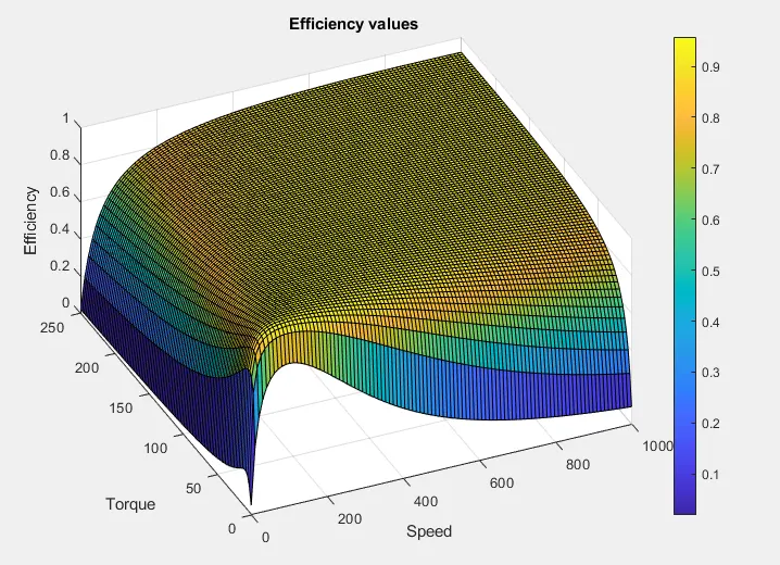
surf(Speed,Torque,Z)
colorbar
xlabel('Speed')
ylabel('Torque')
zlabel('Efficiency')
title('Efficiency values ')
Output
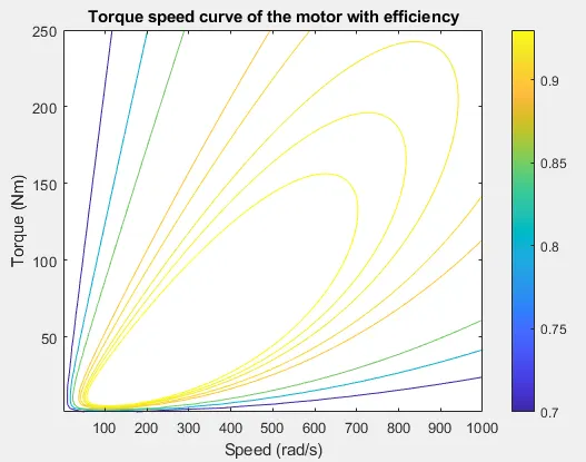
In the contour plot given in the output below the colorbar shows the efficiency values.
In the surf plot, the efficiency of all the points in the torque speed graph is displayed