Week-11 Challenge: Braking

 Study 1:

Braking energy calculation:

A driving cycle is a series of data points representing the speed of a vehicle versus time. Driving cycles are produced by different countries and organizations to assess the performance of vehicles in various ways, as for instance fuel consumption, electric vehicle autonomy and polluting emissions.

 There are different driving cycles, some of them are as follows:

• European Driving cycles
• American Driving cycles
• Japanese Driving cycles
• Global hormanised driving cycles
• Heavy Duty test cycles

1. Automobile energy consumption could be calculated by the use of driving cycles, Electrification of vehilce makes it feasible to recover some of the energy lost in braking.A hybrid braking system was developed to ensure the efficient braking of vehicle and recovering the braking energy.
2. The design and control objectives of such hybrid braking system is to ensure sufficient braking force to quickly reduce the vehicle soeed,properly distributing the brake force to front and rear axle , and also to recover as much as braking energy possible.
3. So understanding of braking energy of a driving cycle is important.

Governing Equation:

Braking Energy = 1/2 mv^2 KWh

Where,

m-mass of vehicle (kg)

v-Velocity of vehicle(m/s)  

Procedure:

• This Driving cycle consists of 24data points and each of these points are used to compute the Braking in a loop fashion.These data points are in the excel format .
• The excel file is then loaded in the matlab using 'xlsread'.
• Speed and time values are extracted.
• Initializing the initial and final speed array.
• Providing the vehicle mass input.
• For loop is used to get the initia and final speed of decelaration 
• Calculating the braking energy by using the formula as shown.
• The graph is plotted for driving cycles and braking Energy.

 Code:

clear all 
close all
clc
%loading the drive cycle
drive_cycle=xlsread('drivec_energy'); 
speed=drive_cycle(:,2); %speed values extracted
time=drive_cycle(:,1);  %time values extracted
vf=[];  %final speed array 
vi=[];  %initail speed array
m=1000; %vehicle mass
for i=1:(length(speed)-1)
    if speed(i)>speed(i+1)
        BE(i)=(0.5.*m.*(speed(i)-speed(i+1)).^2)/3600 %calculating braking energy 
     end
end

fprintf('total braking energy in KWh = %d',sum(BE));
figure(1)
subplot(2,1,1)
plot(time,speed,'linewidth',2)
title('Drive Cycle')
xlabel('Time(sec)')
ylabel('Speed')
grid on


subplot(2,1,2)
plot(BE,'linewidth',2)
xlabel('Time(sec)')
ylabel('Braking Energy(KWh')
grid on

The corresponding braking phenomena taking place at every decelaration condition of the vehicle w.rt to the driving cycle plotted as follows.

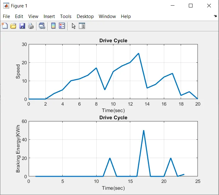
It is very clearly seen from the graph that whenever the vehicle is decelarating from higher initial position to lower final position the braking phenomena is taking place which is shown in the plot. Corresponding to this the Total Braking Energy used by the vehicle is coming out as follows 

 Graph:

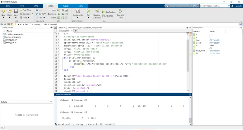
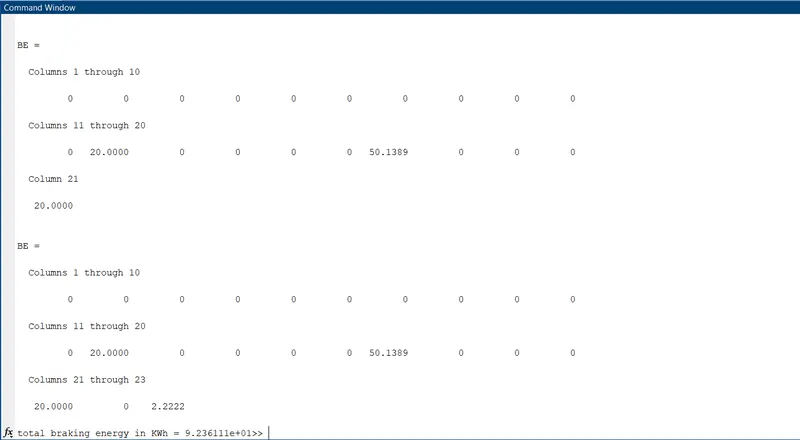
Total braking energy in KWh = 9.236111e+01

Study2:

A)Why electric motor can’t develop braking torque at high speed similar to starting? 

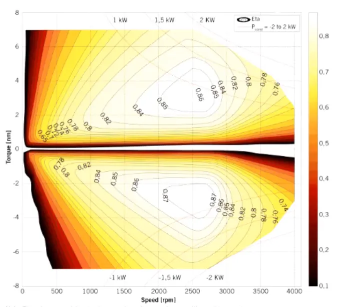
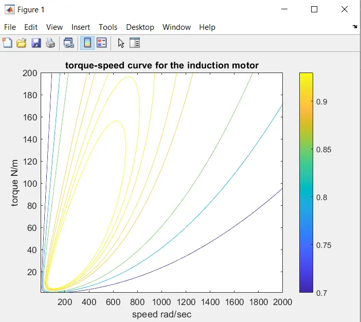
• The figure represents the torque speed variation for a motor. As we can see that the contour obtained is the mirror image.
• The contour lines above the partition is for the torque speed varaition while acceleration.
• The contour lines below the partition is for decelaration or braking case.
• If we extrapolate a point the accelaration region and to the decelaration region , we find the corresponding torque is not same as shown in the fig.
• Hence , the braking torque is not same as that of accelaration torque. The reason would be that once the motor goes down the base speed , the torque is comprimised.
• At high speed while applying the brakes , the brake torque is less compared to the accelaration torque.
• For an EV , regenerative braking will not be effective , as the current back to the battery while braking is less compared to what the battery delivers while accelarating.

B)How electric and mechanical brakes are coordinated? 

Electrical Braking systems are used for funtional braking and mechanical braking systems are used for emergency stopping or for parking.

Electrical Braking is usually very smooth and comfortable and there are no wear from electrical braking. On other hand mechanical braking are usually rough and uncomfrtable and causes wear in th braking components and requires regular maintainence.

It is possible in Electrical braking system to return the regenerated energy back to main supply whereas in mechanical braking it is not possible, and energy is always lost as heat,noise and wear.

Electrical Braking cannot be used as a safety device .Most systems will require a mechanical braking system as a backup safety device.

so in these conditions we use braking strategies were both electrical and mechanical braking is coordinated

Now we have to coordinate between the electrical and mechanical brakes , we will need a strategy to implement the effective brakes.The brake control stratgey are of 2 types.

1. Series: In series, one particular type of brake is applied one after the other i.e regenerative,electric,regenerative etc..

2. Parallel :It can implement both brakes at a time simultaneously.

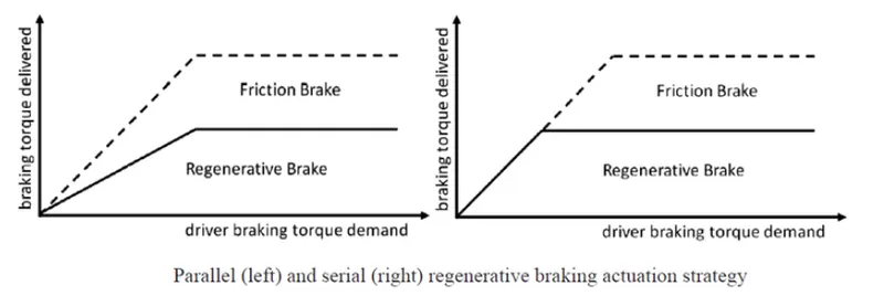
In this strategy, the regenerative braking ratio can be increased in comparison to the parallel braking strategy.

The mechanical brake starts to operate only in the case when the electrical brake reaches its maximum, which is lower than that requested by the driver.

 Study 3:MATLAB program to plot contour of given motor speed, torque and efficiency values.

 To find the effeiciency contoour plot , the motor have different types of losses. They are as follows

Losses:

• Copper losses - kc.T^2
• Iron losses -ki.W
• Windage losses - kw. W^3
• Constant losses

where,

W=speed;

T= torque,

kc - copper loss

ki - iron loss

kw - windage loss

const - constant loss

clear all
close all
clc

%speed & torque array
W= linspace(1,2000,250);
T=linspace(1,200,350);

[X,Y]=meshgrid(W,T)

%loss constants
kc = 0.2;
ki = 0.008;
kw = 0.00001;
const = 20;

%Motor loss calculations
l_copper = (Y.^2)*kc;
l_iron = (X*ki);
l_windage = (X.^3)*kw;

%output power , input power & efficiency calculations
pout = X.*Y;
pin = pout + l_copper+ l_iron+ l_windage + const;
Z = pout./pin
%Efficiency values for contour
V=[0.70,0.80,0.85,0.90,0.91,0.92,0.925,0.93];

figure
box off
grid off
contour(X,Y,Z,V);
colorbar
xlabel('speed rad/sec')
ylabel('torque N/m')
zlabel('Efficiency')
title('torque-speed curve for the induction motor')

figure
surf(X,Y,Z)
colorbar
xlabel('speed rad/sec')
ylabel('torque N/m')
zlabel('Efficiency')
title('Efficiency curve for the induction motor')

Procedure

• Initializing motor speed and torque array values by using linspace command.
• Generating the mesh grid.
• Providing the values for the copper,iron ,windage and constant losses.
• Calculating copper losses , iron losses, windage losses
• calculating the output power.
• Calculating the Input power by adding all the losses and output power.
• Now calculating the efficiecncy 
• Providing the values for mapping efficiency points.
• command for contouring plots 
• Labelling commands for the plots.

Graphs:

Conclusion:

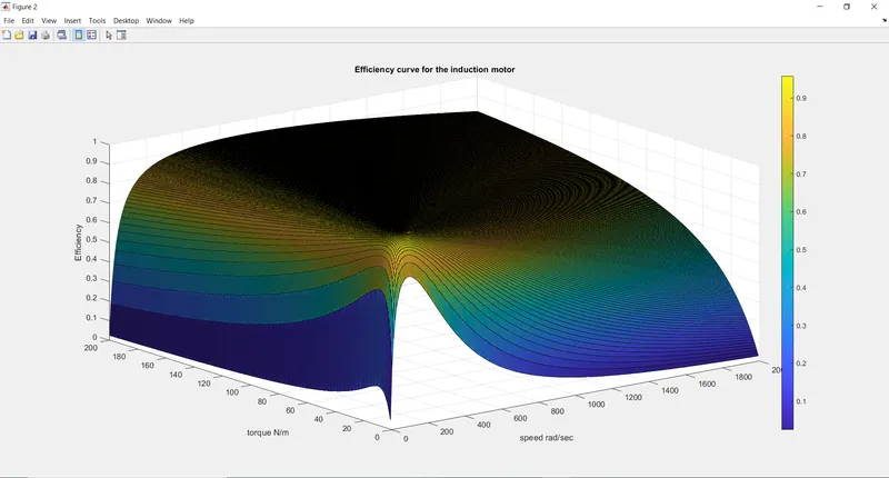
Each of these contours represents efficiency of a particular magnitude which is same over the same contour. It is to be noted that the innermost contour passes the highest efficiency whereas the outermost contour passes the lowest efficiency.