Week-11 Challenge: Braking

Week-11 Challenge: Braking

1) For a defined driving cycle, calculate the energy required for braking.

The powerplant of a vehicle produces power to satisfy tractive effort requirements of acceleration and steady state operation. When it comes to deceleration, driver cannot rely solely on aerodynamic drag to bring vehicle to a stop in required distance. Brakes are used for increasing the rate of deceleration. Brakes use friction to reduce the relative velocity of wheels and the wheel upright to which brake caliper is connected. This in turn slows the vehicle down faster than simply relying on drag. Worldwide harmonized light duty test cycle is used for evaluating braking energy required for vehicle. The vehicle has the following characteristics.

WLTC class 2-

Weight=2000 kg

Drag area=0.65 m²

Drag coefficient=0.3

Standard air density of 1.225 kg/m³ is used for calculating energy lost to drag. Vehicle is assumed to move on a flat surface, without any incline and without losing traction during acceleration or braking. The following plots are obtained.

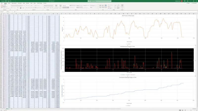
Figure 1-Braking energy

The first plot shows the variation of velocity with time. Velocity is given in m/s and time is in second. The second plot shows the braking energy required by vehicle during deceleration to adhere to required duty cycle. Energy is given in kilowatt-hours and time is in seconds. The green line depicts total energy lost during deceleration, the blue line depicts drag energy loss and red line depicts braking energy loss. All values of energy are given in kilowatt-hours, plotted against time in seconds. In electric and hybrid vehicles a portion of this energy may be used to charge the battery during regenerative braking. The last plot shows the variation of cumulative braking energy lost to surrounding as heat during test cycle. Energy is plotted in kilowatt-hours and time is in seconds. Test lasts for 1477 seconds.

One would expect to see braking energy in graph 2 to have positive value whenever deceleration is required. Observing graph 2 shows that this is not the case. Aerodynamic drag can decelerate the vehicle whenever tractive effort is less than steady state torque requirement. Thus, brakes are only used when deceleration required is more than aerodynamic drag can provide. For every second of travel the difference in past speed and present speed is calculated. Using this energy difference between 2 states is used to calculate energy lost during deceleration using the formula-

Kinetic energy change=0.5*vehicle mass*(difference in squared speed over one second)

If this difference in kinetic energy can be provided by aerodynamic drag, then the brakes do no work, and does not show up on graph 3. If however the drag at that speed is insufficient to decelerate the vehicle in accordance with duty cycle, brakes are engaged and energy lost is reflected in graph 3. Over entire cycle, vehicle loses 0.95 kilowatt-hours of energy to braking.

2) Why electric motor can’t develop braking torque at high speed similar to starting? How electric and mechanical brakes are coordinated?

Torque of a motor varies over its operating speed range as shown below-

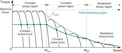
Figure 2-Induction motor torque vs speed

An AC induction motor supplied by a variable frequency drive is capable of high starting torque. This torque can be maintained up to a certain rpm and is called constant torque region of motor operation. Above this speed, armature voltage limits, the power output. In order to produce peak power over the rest of its operating range, torque reduces in an inverse exponential manner as speed increases. This is called constant power region. Above this speed, motor must rely on breakdown torque at individual frequencies to produce appreciable torque. Motor output power starts reducing from peak value and torque begins to fall more sharply than in constant power region. The combined operating range of constant power region and breakdown torque region is known as field weakening region. This is because field flux is reduced for operation in these regions.

When motor is used as a brake, a similar trend is followed. The blue line is mirrored about the horizontal axis and falls in the negative torque region while rotational speed remains positive. If motor is used for braking at high speed, the negative torque produced is in field weakened region and cannot be of equal magnitude to peak torque in constant torque region.

Due to this limitation, friction brakes and electric brakes work in tandem to produce required braking force at all speeds. Friction brakes may be used at high speed and regenerative brakes at low speed. This is called series brake control strategy. The alternative is to use both brakes in parallel. The following graph shows the variation of braking torque produced by electric motor and friction brakes with speed.

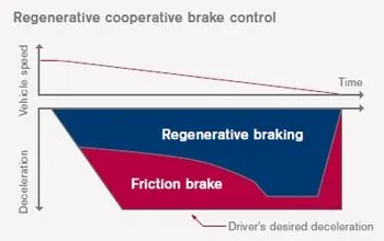
Figure 3-Parallel braking strategy of Nissan Leaf

The graph above shows the braking force produced by friction and regenerative brakes on Nissan Leaf. The leaf uses friction and regenerative brakes in parallel to produce constant torque while maximising regenerated energy fed back to battery. When maximum braking torque is desired by driver at high speed, most of the braking force is provided by friction as braking torque at high speed is poor. As vehicle slows down, regenerative brakes provide most of the braking force as motor enters constant torque regime. The torque bias between the two braking systems is varied constantly so that the brakes don’t lock up under heavy braking. If less than maximum braking torque is desired, friction brakes are used sparingly as the motor alone can provide desired braking torque. Thus, the two braking systems work in parallel to provide necessary braking torque over the entire range of vehicle speed, without exceeding tractive limit of tires.

3) Make a MATLAB program which plots contour of given motor speed, torque and efficiency values. Attach the code as a .m file attach a screenshot of all the plots.

Matlab program for plotting electric motor characteristics is shown below-

clear all
close all
clc
% motor operating range
x=linspace(1,1000); % motor speed range in rad/s
y=linspace(1,250); % motor torque range in N.m
% motor loss constants
kc=0.2; % copper loss
ki=0.008; % iron loss
kw=0.00001; % windage loss
ConL=20; % constant loss
% mesh for plotting efficiency over operating range of motor
[X,Y]=meshgrid(x,y);
Outputpower=(X.*Y); % power=speed*torque
B=(Y.^2)*kc; % copper loss
C=X*ki; % iron loss
D=(X.^3)*kw; % windage losses
Inputpower=Outputpower+B+C+D+ConL;
efficiency=Outputpower./Inputpower;
V=[0.7,0.75,0.8,0.85,0.9,0.91,0.92,0.93,0.94,0.95];
grid off
contour(X,Y,efficiency,V); % plotting contour plot of efficiency over operating range
xlabel('Speed in rad/s');
ylabel('Torque in N.m');

Efficiency of motor is plotted from 1 to 1000 radians per second and 1 to 250 Newton metres of torque. Motor loss constants relating to copper losses, iron losses, windage losses and constant losses are then specified by user. Meshgrid function provides values of torque and speed for all points on 2-dimensional grid. Output power is calculated by multiplying torque with speed at all operating conditions. Iron losses, copper losses and windage losses are then calculated over entire operating range. The input power is calculated by adding the losses to the output power. The efficiency at each point is calculated as the ration between output and input power. Efficiency contour values ranging from 70% to 95% are then stored in variable V to be used in contour command. The contour command connects all points within operating range having the same efficiency. The following contour diagram is obtained as output-

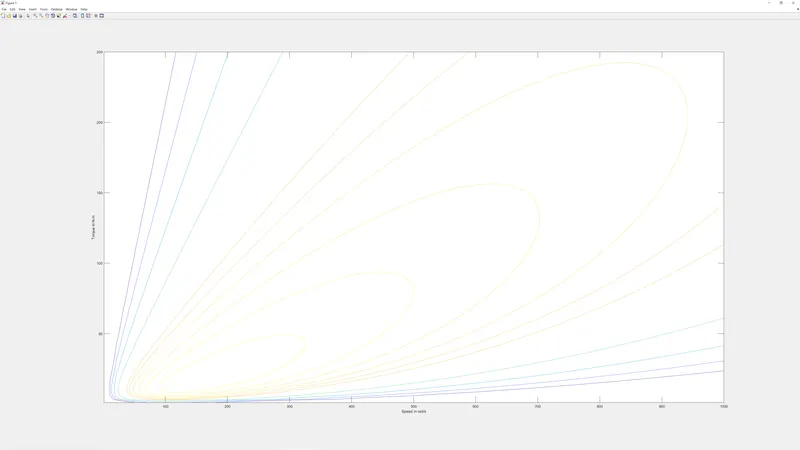
Figure 4-Motor efficiency contour plot

The figure above plots torque in Newton metre on the vertical axis and speed in radians per second on the horizontal axis. We can see that the motor maintains high efficiency, except near the axes. This is because at low power output, constant losses become a large percentage of input power. As output power increases so does the efficiency until iron losses and copper losses become significant. Iron losses occur primarily at high speed and copper losses occur at high torque demand due to current draw. Thus, the motor is most efficient at moderate speed and torque. This is shown by the large efficiency island in the middle of the contour plot.