Week-11 Challenge: Braking

PART 1

AIM: To calculate the energy required for braking in a defined driving cycle.

EQUATIONS USED:

Breaking energy = ½*m*((Vi)^2-( V_f) ^2)

where m is the vehicle's mass and Vi is the speed at the start of braking and Vf at the end of braking.

BODY:

A driving cycle is a series of data points representing the speed of a vehicle versus time. Driving cycles are produced by different countries and organizations to assess the performance of vehicles in various ways.

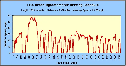
In this calculation, UDDS Drive cycle data is used. The total Braking energy required for the UDDS drive cycle is calculated.

UDDS Drive cycle - The EPA Urban Dynamometer Driving Schedule (UDDS) is commonly called the "LA4" or "the city test" and represents city driving conditions. It is used for light-duty vehicle testing. The UN/ECE Regulation 53 refers to the EPA UDDS as the "Test Equivalent to the Type 1 Test (verifying emissions after a cold start).

The vehicle mass is assumed as 1000 kg and 5 % of vehicle mass is added as the moment of inertia of all rotating parts in the vehicle.

MATLAB CODE:

clear all
close all
clc

% Reading the data from drive cycle text file.
f1 = fopen('uddscol.txt','r');
fgetl(f1); %reading header.
fgetl(f1); %reading 2 line.
A = fscanf(f1,'%f',[2 inf]);
A = A';
time = A(:,1); %time in seconds
v = A(:,2);
velocity = v*0.44704; % mph to m/s

%inputs
mass = 1000 + 0.05*(1000); %kgs
decrease_in_velocity = zeros(1,length(time));
change_in_time = zeros(1,length(time));
deceleration = zeros(1,length(time));
braking_energy = zeros(1,length(time));

%energy calculations
for i = 1:(length(velocity)-1)
    if velocity(i) > velocity(i+1)
        decrease_in_velocity(i) = velocity(i+1) - velocity(i);
        change_in_time(i) = time(i+1) - time(i);
        deceleration(i) = decrease_in_velocity(i)/change_in_time(i);  
        braking_energy(i) = 0.5*mass*0.001*((velocity(i))^2 - (velocity(i+1))^2)/3600;
        
    end
end

%plotting
figure 

subplot(3,1,1)
plot(time,velocity)
xlabel('Time (seconds)')
ylabel('Velocity (m/s)')
title('Urban Dynamometer Driving Schedule (UDDS) drive cycle data')

subplot(3,1,2)
plot(time,deceleration,'r')
xlabel('Time (seconds)')
ylabel('Deceleation (m/s^2)')
title('Decelartion values for UDDS drive cycle data')

subplot(3,1,3)
plot(time,braking_energy,'g')
xlabel('Time (seconds)')
ylabel('Braking enrrgy (kWh)')
title('Braking energy values for UDDS drive cycle data')

fprintf('The total braking energy required for UDDS drive cycle for a time period of %d seconds is %.3f kWh',length(time),sum(braking_energy))

PLOTS:

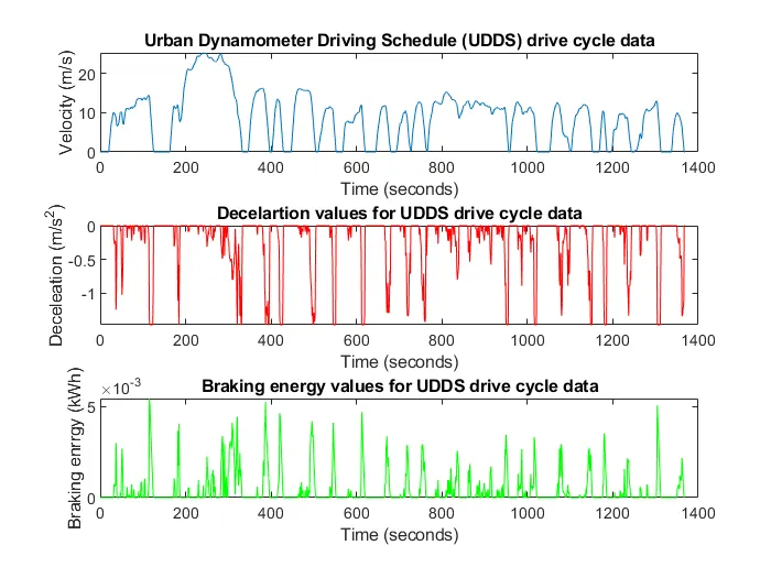
RESULT:

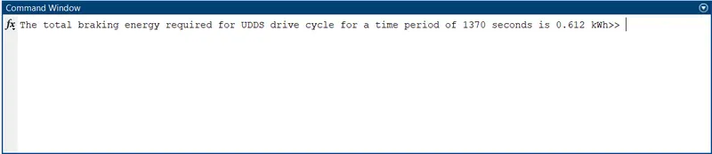
The total braking energy required for the UDDS drive cycle for a time period of 1370 seconds is 0.612 kWh.

PART 2

AIM: To study the braking torque and braking operation.

OBJECTIVE:

1.To find the reason why electric motor can’t develop braking torque at high speed similar to starting.

2.To find how electrical and mechanical brakes are coordinated.

BODY:

1. Electric motor can’t develop braking torque at high speed similar to starting because -

When the motor is at rest and it has to operate from a standstill position to reach the moderate speed, higher torque is required to bring the motor into operation. Whereas when the vehicle is already at high speed the capping or the limit is reached by the motor operation and thus any further higher torque could not be obtained while braking. The braking operation happens in the motion which is been distributed as per proportion in the BRAKE ENERGY and the REGENERATIVE BRAKING.

This situation occurs only when the vehicle is at high speeds because the motor will be running at the constant power region. In the constant power region, the torque of the motor reduces and so the motor cannot develop the braking torque which is equal to the torque that occurred during low speed at the constant torque range.

Moreover, as we know the torque of the induction motor is inversely proportional to the square of the rotor speed. So, at high speed, the torque will be less. That’s why at high speed, the electric motors cannot produce braking torque similar to starting.

2. Breaking

Electrical breaking

Electrical braking can be done by many methods such as Unbalancing the input points of current to the motor, Using transistors in the H-bridge arrangement to reverse the motor direction in order to reduce speed, Implementing a regenerative braking system by using bi-directional power converters. Regenerative braking converts much of the energy to electrical energy, which may be collected for later use.

Mechanical breaking

In Mechanical braking which we usually see and experience in all vehicles, the brake pedal in the vehicle cabin helps us to engage or disengage the brakes.

These brakes commonly use friction between two surfaces pressed together to convert the kinetic energy of the moving object into heat, though other methods of energy conversion may be employed. The friction between the surfaces is performed using pressurized air or pressurized oil which are commonly known as an air brake and hydraulic brake respectively.

Coordination between electrical and mechanical breaks.

Two types of brake control strategies are used to organize the electrical brake and mechanical brake they are, Series control strategy and Parallel control strategy.

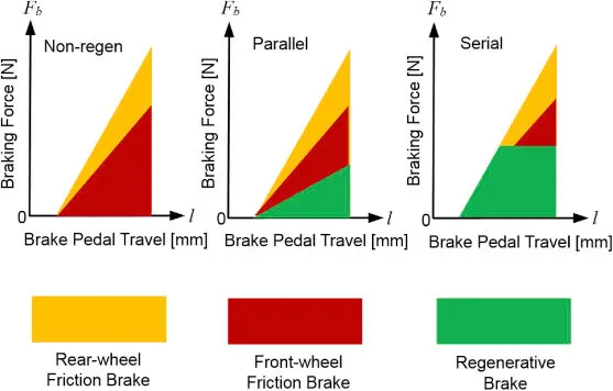
Series control strategy - The Regenerative Braking or the Mechanical Braking both are applied one after another.

Parallel control strategy - The Regenerative Braking or the Mechanical Braking both are applied Parallelly.

Example

EDIB is a brake control strategy which is developed by NISSAN. It is a type of parallel braking.

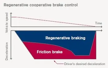
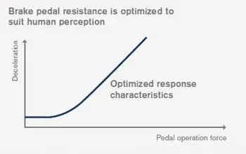
It controls the regenerative brake and friction brake to support both of these requirements. Further, it also controls the reactive force from the pedal in order to unify the feeling when stepping down on the pedal and the sense of deceleration.

At low speed the torque of the motor is high and so the regenerative brake has a higher braking part than the frictional brakes.

RESULT:

At higher speeds, the frictional brake is used to slow down the vehicle, the rear-wheel frictional brake will be employed if the braking requirement is not fulfilled then the front wheel frictional brake is also used and a small amount of regenerative braking is used simultaneously or later depending on the configuration being parallel or series.

PART 3

AIM: To plot contour of given motor speed, torque, and efficiency values.

EQUATIONS USED:

Total losses = K_cT² + K_iW + K_wW³ + C;

Where,

Kc = Copper loss constant

Ki = Iron loss constant

Kw = Windage loss constant

C = constant losses

T = Torque of the motor

W = Speed of the motor

BODY:

As we know “Energy neither can be created nor it can be destroyed, it can only be transferred from one form to another”. In a DC machine, mechanical energy is converted into electrical energy. During this process, the total input power is not transformed into output power. Some part of input power gets wasted in various forms. The form of this loss may vary from one machine to another. These losses give in rise to the temperature of the machine and reduce the efficiency of the machine.

These losses are-

1. Copper losses

The copper losses are the winding losses taking place during the current flowing through the winding. These losses occur due to the resistance in the winding. In a DC machine, there are only two windings, armature and field winding.

These losses are I²R losses but can be represented in the form of K_cT², where K_c is copper loss constant and T is the torque.

2. Iron Losses

As the iron core of the armature is rotating in the magnetic field, some losses occur in the core which is called core losses.

These losses can be represented in the form of K_iW, where K_i is the iron loss constant and W is the speed.

3. Windage Losses

Windage is a force created on an object by friction when there is relative movement between air and the object. Windage loss is the reduction in efficiency due to windage forces. Electric motors are affected by friction between the rotor and air.

These losses can be represented in the form of K_wW³, where K_w is windage loss constant and W is the speed.

4. Extra constant Losses

There are some more losses. These losses are called stray-load losses. These miscellaneous losses are due to the short-circuit current in the coil undergoing commutation, distortion of flux due to the armature, and many more losses. These losses are difficult to determine and often found experimentally and represented by C.

So total losses can be represented as,

Total losses = K_cT² + K_iW + K_wW³ + C;

MATLAB CODE:

%Speed vs Torque for different efficiencies
clear all
close all
clc

W = linspace(0,1000); %speed in rad/sec
T = linspace(0,300); %torque

%motor loss constants
kc=0.18; %For copper losses
ki=0.006; %For iron losses
kw=0.000015; %For windage losses
conL=20; %For constant motor losses

%Meah generation
[X,Y]=meshgrid(W,T);

%calculations
Outputpower=(X.*Y); %Torque x speed = power
B=(Y.^2)*kc; %Copper losses
C=(X*ki); %iron losses
D=(X.^3)*kw; %Windage losses
Inputpower = Outputpower + B + C + D + conL;
Z = Outputpower./Inputpower; %Calculated efficiency

% Efficiencies for contour
V=linspace(0.7, 0.95, 10);

%Plotting the contour
box off
grid off
contourf(X,Y,Z,V);
xlabel('Speed/rad.s^-^1');
ylabel('Torque/N.m');

%end of the program

RESULT:

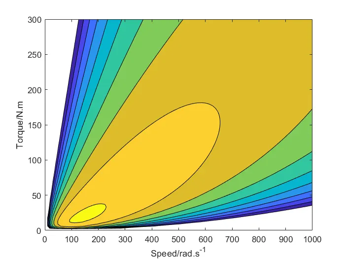
As we can see at low speeds the torque is more than compared to high speeds and also maximum efficiencies occur at average speeds.

SOURCES:

https://www.electrical4u.com/losses-in-dc-machine/