Week-11 Challenge: Braking

1. The objective is to calculate the energy required for braking for a defined driving cycle.

• Driving Cycle is a plot of data points where the speed of the vehicle is plotted with respect to time. There are many defined standards of Drive cycles across the world. For our case, the FTP75 drive cycle is used to calculate the braking energy.
• Cold start transient phase (ambient temperature 20-30°C), 0-505 s,
• Stabilized phase, 506-1372 s,
• Hot soak (min 540 s, max 660 s),
• Hot start transient phase, 0-505 s.

• Duration: 1877 s
• Distance traveled: 11.04 miles (17.77 km)
• Average speed: 21.2 mph (34.12 km/h).
• Maximum speed: 56.7 mph (91.25 km/h).

• Kinetic Energy can be derived from the formula,

E = 1/2 *m*v^2

where,

E = Energy

m = mass of the vehicle

v = Velocity of the vehicle after braking

• Here, there are two velocities, one is the initial velocity and the other one is the final velocity after braking is performed.
• So the two velocities are taken into account for energy calculation.

E = 1/2 * m * ((V1)^2 - (V2)^2)

where,

m = Mass of the Vehicle

V1 = Initial velocity

V2 = Final velocity

• Let's assume that the mass of the vehicle is 2000kg.
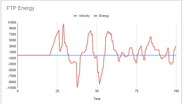
• The Energy is calculated for 100 sec for the FTP drive cycle and the values are plotted in the graph.

https://docs.google.com/spreadsheets/d/1oFICAG95bFWBg7HdrMHG7S3Pd6jR1uHqcG2WstgI4d0/edit?usp=sharing

2. The objective is to identify why electric motor can’t develop braking torque at high speed similar to starting and how electric and mechanical brakes are coordinated.

• Basically, the torque and speed characteristics are not the same during motoring and braking operations.
• We know that Torque is inversely proportional to Speed so that if speed increases torque decreases.
• There is two Torque acting in the vehicle such as Starting Torque and Braking Torque.
• Starting Torque: Speed is low in the initial condition of the vehicle, and Initial Torque is high
• Braking Torque: Speed increases and are at a high value, and when braking, the speed decelerates. Due to the high value of speed, the braking torque produced is of low value.
• Thus, the electric motor can’t develop braking torque at a high speed similar to starting due to the above-stated factor.

Electric and mechanical brakes are coordinated Brake Strategy Subsystem

• As far as braking Torque is concerned, the vehicle does not have enough braking torque to stop the vehicle during Braking.
• So, during the initial phase of braking, the mechanical brakes take place until the braking torque catches up to the value.

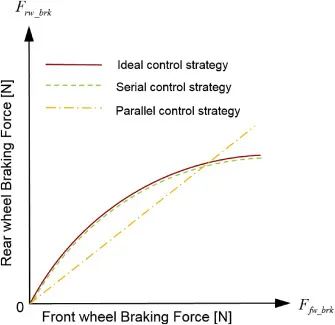
There are two types of Brake Strategy Subsystem

• Series Brake Strategy
• Parallel Brake Strategy

Series Brake Strategy

• Let's consider the vehicle is front-wheel-driven and during the braking operation, it checks some conditions and performs the necessary braking operations.
• When the brake pedal is pressed, with the consideration of the level of depression a braking torque request is sent.
• Firstly, it checks that the state of charge is greater than 80% which is set to be the Threshold level for regenerative charging
• If it is equal to (or) greater than 80 %, then the brake applied to the front axle and back axle is distributed according to the required percentage.
• If the Soc is lesser than 80%, then the brake Torque request is compared with the maximum Regentaive torque.
• If the overall brake torque request is lesser than the maximum regenerative torque of the vehicle, then the braking is done by regenerative braking and the battery is charged.
• If the requested overall brake torque is greater than the maximum regenerative torque of the vehicle, the braking is applied via mechanical braking where the battery is not charged.
• Since the vehicle is front-wheel drive if the brake torque request from the front wheel is lesser than the maximum regenerative torque of the vehicle, then the front brakes are purely applied via regenerative braking and rear brakes are applied via friction.
• The vehicle is front-wheel drive if the brake torque request from the front wheel is greater than the maximum regenerative torque of the vehicle, then the front brakes are applied via ( Regenerative braking + Mechanical Braking ) and rear brakes are applied via friction.

Parallel Brake Strategy

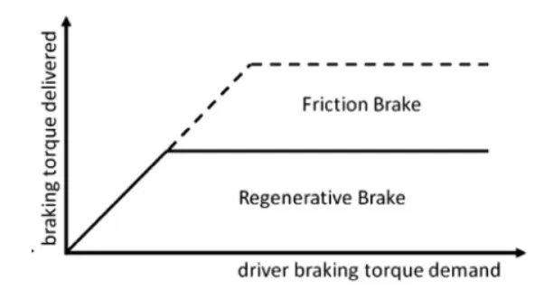
• The Parallel brake Strategy, consists of an electrical and mechanical braking system. This system has a clear division of brake applied via electrical and friction braking.
• The braking forces are applied in parallel and simultaneously where the regen brakings are only done in the front wheel axle.
• The mechanical brake has a fixed ratio for a brake force distribution to the front and rear axle.
• If the overall brake torque request is lesser than the maximum regenerative torque of the vehicle, then the braking is done by Mechanical braking on the rear axle and (Regenerative braking + Mechanical Braking) is applied on the front wheel and the battery is charged.
• A Pressure sensor senses the demanded deceleration torque using hydraulic pressure in the cylinder.
• Then the pressure signal is sent to the motor's controller to actuate the braking operation after checking certain conditions.
• Comparing with Series brake Strategy, this one is much more efficient and simple to operate.

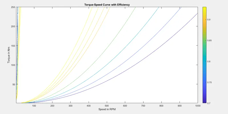
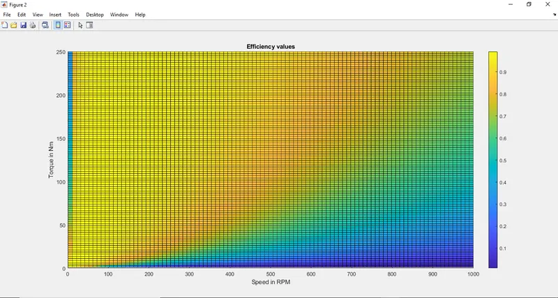
3. The objective is to make a MATLAB program that plots the contour of given motor speed, torque, and efficiency values.

• To plot the contour of motor speed, the input power, and output power must be calculated.
• The input power consists of losses during the motoring operation.

Four losses take place in the power distribution to the motor.

• Copper Loss: (T^2) * Kc
• Iron Loss: w * Ki
• Windage Loss: (w^3) * Kw
• Constant Motor Loss.

where,

T = Torque in Nm

w = Speed in rad/sec

Kc = Coefficeint of Copper Loss

Ki = Coefficeint of Iron Loss

Kw = Coefficeint of Windage Loss

• The Speed and Torque values of the motor are set and the efficiency range is also included.
• By mesh grid, we can plot the characteristics from 1D to 2D representation.

clc
clear all

W=linspace(1,1000);
T=linspace(1,250);

Kc= 0.2
Ki= 0.008
Kw= 0.0001
C= 20

[X,Y] = meshgrid(W,T);
Outpower = (X.*Y);

Copperloss = (Y.^2) .* Ki;
Ironloss = X .* Ki;
Windageloss = (X.^3) .* Kw;


InputPower = (Outpower + Copperloss + Ironloss + Windageloss);
Efficiency = Outpower ./InputPower;
    
W=[0.7,0.75,0.8,0.85,0.9,0.91,0.92,0.93];




contour(X,Y,Efficiency,W)
colorbar
xlabel('Speed in RPM') 
ylabel('Torque in Nm')
zlabel('Efficiency')
title('Torque-Speed Curve with Efficiency')



figure
surf(X,Y,Efficiency);
colorbar
xlabel('Speed in RPM')
ylabel('Torque in Nm')
zlabel('Efficiency')
title('Efficiency values') 

• The results are given below,