Week-11 Challenge: Braking

Qn.1)For a defined driving cycle, calculate the energy required for braking.

Let us consider a arbitrary driving cycle:

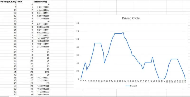
From the graph, let us analyse few instants of braking to find the braking energy.

1.) 41 Km/hr to 31 Km/hr in 5 seconds

2.) 90 Km/hr to 40 Km/hr in 4 seconds

3.) 116 Km/hr to 25 Km/hr in 22 seconds

4.) 55 Km/hr to 0 Km/hr in 8 seconds

6.) 50 Km/hr to 0 Km/hr in 9 seconds

Braking Energy is given by the expression,

`E_b= 1/2* M. (V_i^2-V_f^2)`

where `E_b`is the braking energy.

`M` is the mass of the vehicle.

`V_f`is the final velocity

`V_i`is the initial velocity

By doing the calculation in the excel sheet,

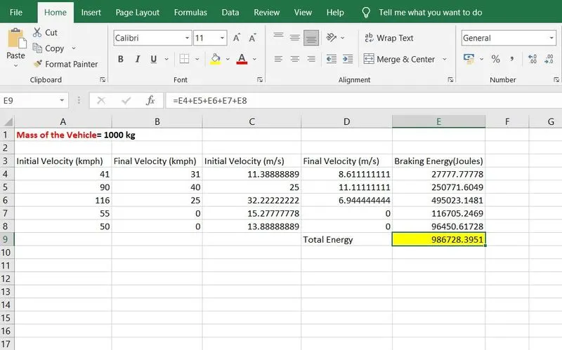
Hence the total braking energy is obtained as 986.72 KJ for the corresponding driving cycle.

Qn.2) Why electric motor can’t develop braking torque at high speed similar to starting? How electric and mechanical brakes are coordinated?

Regenerative braking in electric vehicle is employed to feed back the energy during deacceleration as a effect of motor acting as generator. They are typically used to extend the range of EVs.

But there are some limitations in this phenomenon. They are:

• The regenerative braking torque CANNOT be made large enough to provide all the required braking torque of the vehicle because it will affect the stability of the vehicle.
• At high speeds, the vehicle might be in the constant power mode which causes less values of the torque produced and this limits the amount of braking torque that is used for regeneration.
• During regeneration, the battery has to be charged. But generally, the rate of charging of battery is much lesser than the rate of discharge of battery. This also limits braking torque at high speeds.
• Regenerative braking also needs bidirectional inverters. High regenerative braking torque reduces the effectiveness of the inverter.

Due to the above said reasons, generally in EVs, for effective braking at high speeds, combination of mechanical braking and regenerative braking is used.

Thus, the cooperation between the mechanical braking system and regenerative braking system is a main part of design of EV braking strategy and it is known as torque blending.

There are two different brake control strategies. They are:

1. Series Control Strategy

2. Parallel Control Strategy

Series Control Strategy

• Here, the combination of mechanical braking system and the regenerative braking system are operated one after the other through an intergrated control.
• Series control strategy could give an increase of 15-30% in fuel efficiency and has more consistent braking due to good torque blending capability.

Parallel Control Strategy

• Here, the combination of mechanical braking system and the regenerative braking system are operated simultaneously without an intergrated control.
• The regenerative force is added to the mechanical force which cannot be controlled.
• The regenerative torque is determined by considering the motor capacity, battery SOC and the vehicle velocity. The regenerative braking force is calculated from the brake control unit by comparing the demanded brake torque and the motor torque available.

Special Control Strategy: Electric Driven Intelligent Brake (EDIB) in Nissan Leaf

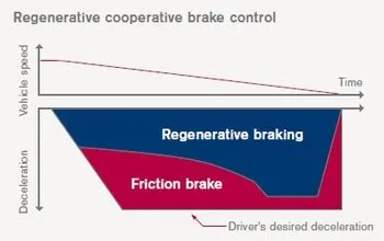
• The braking control is split between regenerative braking and mechanical braking based on the speed so as to achieve the best possible results.
• In EDIB, at low speeds, Regenerative braking is higher (80%).
• At higher speeds, the total braking torque is contributed by 40% regenerative braking and 60% mechanical braking(Fricton brake)

The below diagram shows the distribution based on the speed:

Qn.3) Make a MATLAB program which plots contour of given motor speed, torque and efficiency values. Attach the code as a .m file attach a screenshot of all the plots.

Let us consider,

Motor speed from 0 to 2000 rpm and

Motor torque from 0 to 1000 Nm

The Motor Constants are:

• Copper loss constant Kc=0.1
• Iron loss constant Ki=0.001
• Windage loss constant Kw=0.0001
• Motor loss constant Cm=25

Script:

clear all
close all
clc
%Defining Speed and Torque
sp=linspace(0,2000,500);
tq=linspace(0,1000,200);
%Defining Motor Constants
kc=0.1; %Cu Loss constant
ki=0.001; %Iron Loss Constant
kw=0.0001; %Windage Loss constant
cm=25; %Motor loss constant
[X,Y]=meshgrid(sp,tq); %obtaining 2-D grid for speed and torque
Pout= X.*Y; %Output power is the product of speed and torque
total_loss=((Y.^2).*kc)+(ki.*X)+((X.^3).*kw)+cm; %Total loss
Pin= Pout+ total_loss;
eff= Pout./Pin; %Efficiency calculation
%Defining efficiency levels of contouring
EL=[0.70,0.72,0.75,0.77,0.79,0.80,0.81,0.82,0.83,0.84,0.85,0.86,0.87,0.88,0.89,0.90,0.91,0.92,0.93,0.95];
%Plotting the efficiency with respect to speed and torque
contourf(X,Y,eff,EL)
colorbar
xlabel('Speed (rpm)');
ylabel('Torque (rpm)');
title(' Efficiency Contour');

Explanation:

The motor constants are initialised and the total loss is calculated from the general loss equation. Finally, the efficiency is computed and then the contour is plotted.

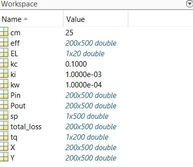
Matlab workspace:

Output Plot:

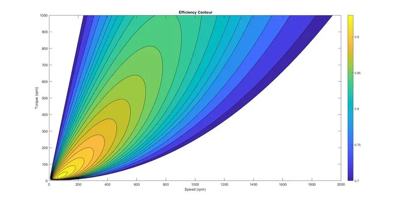
Hence, we could see the regions where we could get high efficiency and operate the motor accordingly.