Week-11 Challenge: Braking

Problem statement:

1. For a defined driving cycle, calculate the energy required for braking.
2. Why electric motor can’t develop braking torque at high speed similar to starting? How electric and mechanical brakes are coordinated?
3. Make a MATLAB program which plots contour of given motor speed, torque and efficiency values. Attach the code as a .m file attach a screenshot of all the plots.

Solution:

1.Drive cycle brake energy calculation:

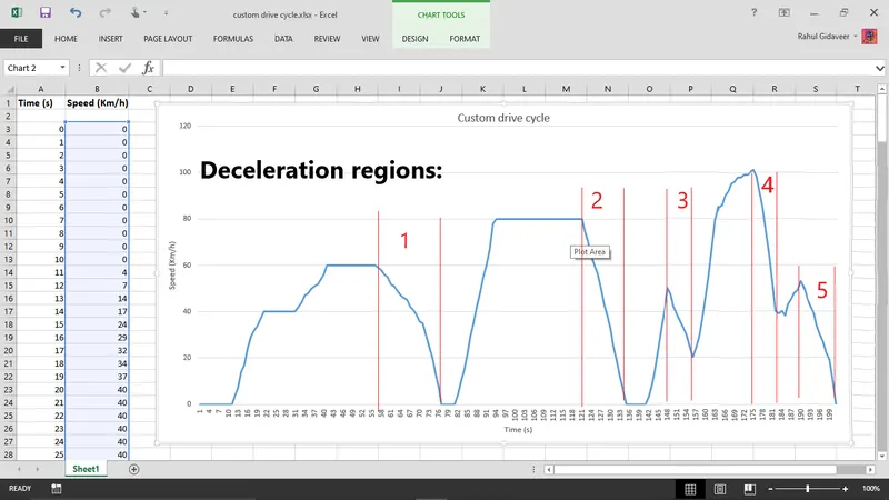
A custom drive cycle is selected for this calculation as shown in the figure below. The deceleration parts are marked.

Procedure for brake energy calculation:

• Identify the region in the drive cycle curve wherein the vehicle is decelerating.
• Obtain the initial speed and time at the beginning of deceleration and final speed and time at the end of deceleration. Calculate the difference between both speed and time values.
• Multiply half the mass of vehicle to the speed difference to obtain brake energy.
• Repeat the above steps at all regions of deceleration and obtain cumulative brake energy and cumulative time of deceleration.
• Divide total brake enery with time to obtain brake power.

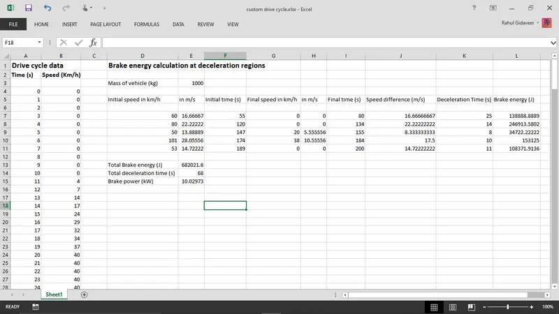
Calculations performed in excel and result is displayed below:

2. Coordination of electric and mechanical brakes:

The braking force is distributed between the electric brakes: Regenerative brakes and mechanical brakes: friction brakes in different ways. Consider an electric vehicle with front-wheel drive. Since the motor is available at the front axle, regenerative braking is also available at the front axle. While friction brakes are available for both axles. The strategies for such distribution are given below:

1. Series brake (optimal feel) :

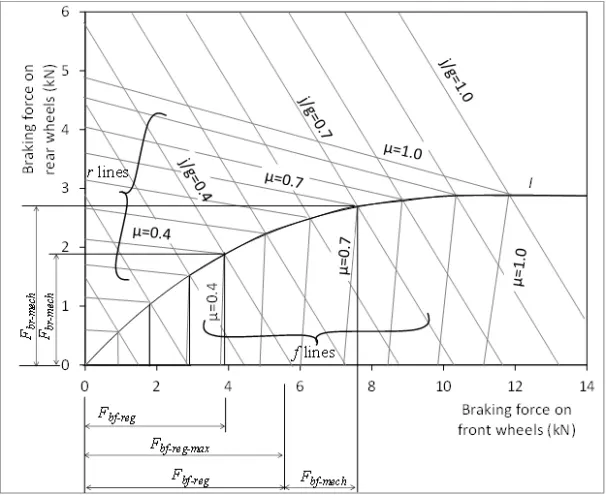
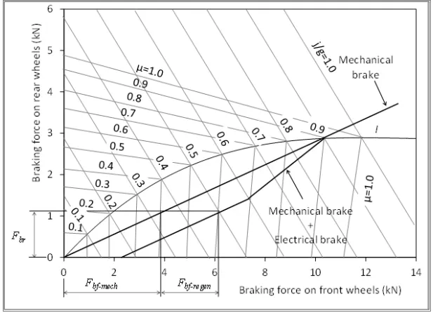
• Series brake is a kind of braking in which the regenerative brakes and friction brakes are applied one after the other. In this kind of distribution, the objective is to minimize the stopping distance. This control strategy is pictorially displayed below. 'j/g' represents the deceleration rate, `mu` represents the road adhesion coefficient.
• When the required deceleration rate (as indicated by the brake pedal position) is less than 0.2 g then only regenerative brakes are applied at front wheels shown by the horizontal solid line on x-axis. If the deceleration rate is higher than 0.2g then brake distribution follows the solid curve line.
• At the front wheel, the braking force is divided between friction brakes and regenerative brake. If the required braking force is less than and equal to the maximum braking force that can be produced by an electrical motor, then regenerative brakes supply the total braking force. And if the braking force demanded is greater than the maximum regenerative torque then the surplus braking force required is provided by friction brakes.
• The maximum regenerative torque is speed dependent. At speeds lower than the base speed, regenerative torque is constant and then it drops continuously beyond base speed. Accordingly the mechanical braking force also adjusts.

2. Series brake (optimal regeneration):

• In this kind of braking strategy, the focus is on the maximum energy recovery from the vehicle kinetic energy.
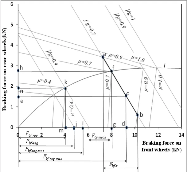
• At point f, the deceleration rate j/g is equal to road adhesion coefficient. In this case, maximum regenrative braking that could be produced by the motor is applied and the surplus force is provided by the mechanical brakes. At the rear wheels, mechanical braking force corresponding to point h is provided. At this point, braking feel and maximum regeneration happens.
• At point c, demanded deceleration is higher than allowable traction at road-tyre interface. In this condition, braking force corresponding to that maximum traction available at wheels can be applied. Since braking force value reduces with reduction in road adhesion, the total force at front axle is provided by regenerative brake.
• At point k, the deceleration and adhesion values are low, only regenrative brakes are applied at front wheels. And braking force on rear follows the curve I.

3. Parallel brake:

Parallel braking is a kind of braking strategy, where both mechanical and electrical brake are put to work simultaneously. Hence the brake feedback available to driver and regeneration of power is conpromised.

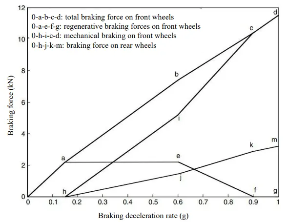
The following features of the parallel brakes are depicted by the figure below:

• At low deceleration rate up to 0.15g, the braking force at rear wheels is zero (0-h). And at front axle, the braking force required is equally and simultaneously provided by mechanical and regenerative brakes.
• Point a indicates the maximum braking force that can be provided by regenrative brakes according to the maximum torque of the motor. If driver further depresses the brake pedal, regenrative brakes cannot provide any greater braking force and rear mechanical brakes come into play. Up to decelration rate of 0.6 g, regenerative braking force remains contant at maximum, while mechanical braking force increases at both axles.
• When the demanded brake output increases beyond 0.6g, the regenerative braking share is reduced up to 0.9g. This indicates emergency braking, wherein the vehicle is required to stop immediately. As the regenerative brake has limitation and is slow in nature, it is not deployed.
• At deceleration beyond 0.9g, no regeneration is allowed and mechanical brakes at both axles take over.

Reference:

• https://nptel.ac.in/content/storage2/courses/108103009/download/M11.pdf