Challenge: Braking

Question

Answers

#1

Braking Energy Calculation

Braking Energy, `E = 1/2M(V_f^2 - V_i^2)`

Where,

Mass of the vehicle, `M = 1450 kg`

Final Velocity in m/s, `V_f`

Initial Velocity in m/s, `V_i`

Shown below is the excel sheet with the drive cycle data and the calculation,

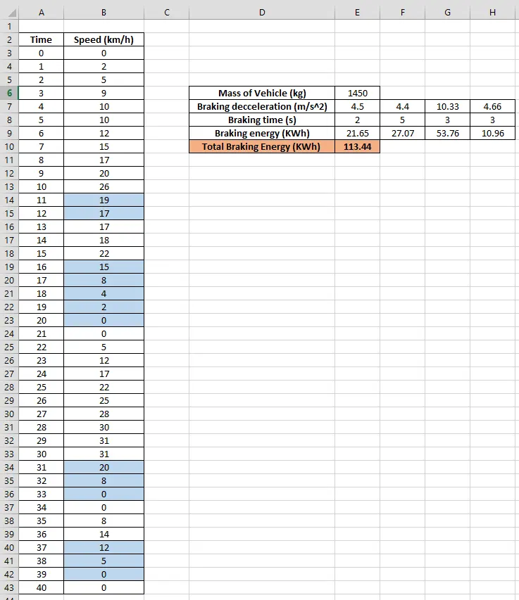
The drive cycle duration is 40 seconds. The total braking energy calculated for the drive cycle from the excel sheet is 113.44 KWh.

MatLAB program to calculate the total braking energy for the same drive cycle.

close all
clear all
clc

%read drive cycle data from excel sheet
data = xlsread('brake_drive_cycle');
time = data(:,1);   %time in seconds
vel = data(:,2);    %speed in seconds
mass = 1450;        %mass of the vehicle

brake_energy = 0;

%Loop to calculate the braking energy
for i=2:time(end)+1
    if vel(i) < vel(i-1)
        brake_energy = brake_energy + (0.5*mass*((vel(i)*5/18)^2-(vel(i-1)*5/18)^2));
        energy(i) = (0.5*mass*((vel(i)*5/18)^2-(vel(i-1)*5/18)^2))/-1000;
    else
        energy(i)=0;
    end
end

%To convert braking energy to KWh as the energy obtained is -ve and in Wh
brake_energy = brake_energy/1000*-1;    

%To display the braking energy onto the command window
fprintf('Total Braking Energy = %3.2f KWh',brake_energy) 

%Plot
yyaxis left
plot(time,vel,'linewidth',2,'color','b')
xlabel('Time - seconds')
ylabel('Speed - km/h','color','b')
yyaxis right
plot(time,energy,'linewidth',1.5,'color','r')
ylabel('Braking Energy - KWh','color','r')
title('Drive Cycle with Braking energy')
legend('Speed - km/h','Braking energy - KWh','location','northwest')
grid on

The below code shows the calculation of braking energy,

brake_energy = brake_energy + (0.5*mass*((vel(i)*5/18)^2-(vel(i-1)*5/18)^2));

where, brake_energy is a variable that saves the total brake energy after each second of the drive cycle.

energy(i) = (0.5*mass*((vel(i)*5/18)^2-(vel(i-1)*5/18)^2))/-1000;

whereas, energy is an array that saves the braking energy for each second at different values of i.

Results

Plot obtained from the MatLAB program is shown below,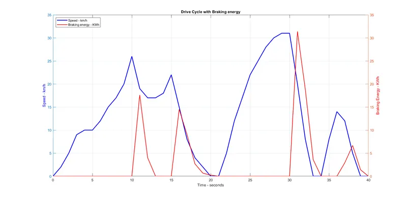

The Plot reprensent both the drive cycle (represented by blue curve) and the braking energy (represented by red curve) of the vehicle.

Shown below is the result obtained in the command window,

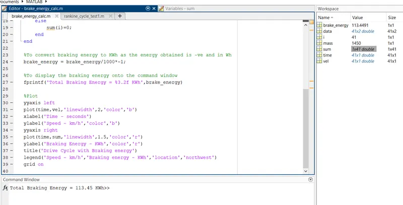
Total Braking Energy Obtained = 113.45KWh

The result from the MatLAB calculation and the Excel calculation are same with a small difference of 0.1KWh, obtained due to rounding off during calculations.

#2

Shown below is the Efficiency and Torque characteristics of an induction motor. The regions shown are of Forward Motoring and Forward Braking operations,

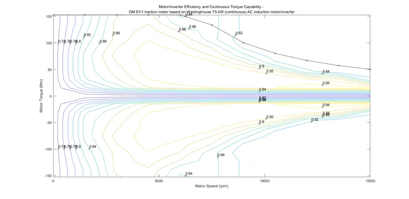
From the above figure it can be understood that the torque-efficiency curves of both operation are different. Electric motors have high starting torque, almost constant torque available at lower speed (speeds below base speed) and at higher speeds (speeds above base speed) this torque tends to decrease hyperbolically, this applies to all the operating quadrants of the motor. For this reason electric motors does not develop braking torque at high speed similiar to starting torques.

Brake Control Strategy

There are two types of brake control strategies - Series Braking and Parallel Braking.

In Series braking, either regenerative brakes are used or mechanical brakes are used at a time. Here the brakes can work in two ways either for efficiency where maximum energy is recovered or for the comfort of the occupants by reducing the jerk caused by braking, this in turn affects the energy recovery.

In Parallel braking, both regenerative brakes and mechanical brakes are used at the same time. Therefore the energy recovered by the system will be small but the braking power will be maximum.

During regenerative braking, the kinetic energy of the vehicle is converted into electrical energy by means of electric motor and it is stored in batteries for later use. Usually regenerative brakes are combined with mechanical brakes to meet the total braking force demand. A controller is used to achieve the balance between regenerative and mechanical brakes. Regenerative brakes are controlled electrically by the control of motor torque and the mechanical brakes will be hydraulically actuated.

In most of the case, regenerative braking is applied at first to slow down the vehicle. When more braking power is required then the mechanical brakes come into play. Regenerative brakes are not very good at proving stopping power at low speeds, during such times they are not used. Moreover regenerative brakes provide high energy recovery in cities than on highway because of the need for constant braking. Therefore they provide an improved fuel efficiency in the range of 20% to 40%. The energy recovery depends on the size of the motor and the efficiency of the control system.

#3

The governing constants and equations

Copper loss constant `= k_c`

Iron loss constant `= k_i`

Windage loss constant `= k_w`

Constant Loss of motor `= conL`

Copper loss is given by `cu = k_cxx(To rque)^2`

Iron loss is given by `I = k_ixxSpeed`

Windage loss is given by `W = k_wxx(Speed)^3`

Power of the motor is given by `Power = To rque xx Speed`

MatLAB program to plot the contour of given motor speed, torque and efficiency values,

clear all
close all
clc

x = linspace(1,1150);           %Speed range - rad/s
y = linspace(1,250);            %Torque range - Nm

%constants
kc = 0.14;                      %Copper loss constant
ki = 0.007;                     %Iron loss constant
kw = 0.000035;                  %Windage loss constant
conL = 80;                      %Constant motor loss

[X,Y] = meshgrid(x,y);          %Create mesh
Pout = (X.*Y);                  %Power = Torque x Speed
B = (Y.^2)*kc;                  %Copper loss
C = X*ki;                       %Iron loss 
D = (X.^3)*kw;                  %Windage loss
Pin = Pout + B + C + D + conL;  %Total input power
Z = Pout./Pin;                  %Efficiency

V = [0.70,0.80,0.85,0.90,0.91,0.92,0.93];

%plot
contour(X,Y,Z,V);
xlabel('Speed - rad/s');
ylabel('Torque - Nm');
hold on
grid off
title('Torque - Speed Contour')

Here, V is an array that holds the different values of efficiency curves required.

V = [0.70,0.80,0.85,0.90,0.91,0.92,0.93];

It currently contains 7 efficiency ranges. So when the contour is plotted, these efficiency ranges will be used to draw the curves.

contour(X,Y,Z,V);

Here, the X,Y and Z represents the x-axis, y-axis and the z-axis respectively. The x-axis represents the motor speed, y-axis represents the motor torque and the z-axis presents the motor efficiency. The V represents the efficiency range in the contour.

Plot

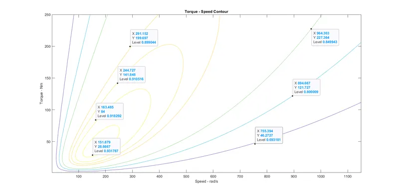
The Torque-Speed contour of the motor obtained is as follows,

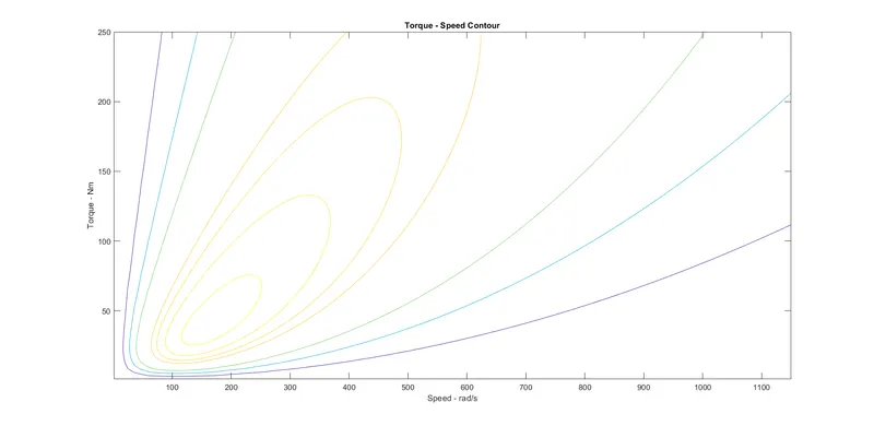
The inner most line and the area inside it represents 93% motor efficiency.

The second line and the area inside it represents 92% motor efficiency.

The third line and the area inside it represents 91% motor efficiency.

The fourth line and the area inside it represents 90% motor efficiency.

The fifth line and the area inside it represents 85% motor efficiency.

The sixth line and the area inside it represents 80% motor efficiency.

The outer most line and the area inside it represents 70% motor efficiency.