Rankine cycle Simulator

Aim: Simulation of an Ideal Rankine Cycle based on user inputs.

Theory: The Rankine cycle is a model used to predict the performance of steam turbine systems commonly found in thermal power generation plants. It was also used to study the performance of reciprocating steam engines. It is an idealized thermodynamic cycle of a heat engine that converts heat into mechanical work while undergoing phase change. Power generation depends on the temperature difference between a heat source and a cold source. The higher the difference, the more mechanical power can be efficiently extracted out of the heat energy.

The efficiency of the Rankine cycle is limited by the high heat of vaporization of the working fluid.

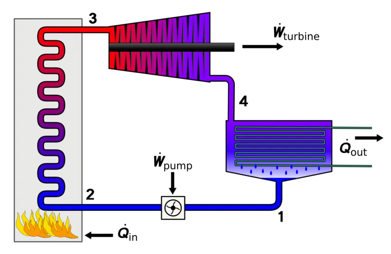
The ideal rankine cycle consists of a pump, boiler, turbine and condenser. Here the friction losses in each of the 4 components are neglected and the heat is supplied externally to a closed loop, which usually uses water as working fluid.

Process in Rankine cycle

There four processes in the Rankine Cycle, they are

Process 1-2: Isentropic compression, here the working fluid is pumped from low to high pressure. Little input energy is required by the pump as the fluid is a liquid at this stage.

Process 2-3: Constant pressure heat addition, the high pressure liquid enters a boiler where it is heated at constant pressure by an external heat source to become a dry saturated vapour.

Process 3-4: Isentropic expansion, the dry saturated vapour expands through a turbine, generating power. This decreases the temperature and pressure of the vapour.

Process 4-1: Constant pressure heat rejection, the wet vapour then enters a condenser where it is condensed at a constant pressure to become a saturated liquid.

In an ideal Rankine cycle the pump and turbine would be isentropic, that is, the pump and turbine would generate no entropy and hence maximize the net work output. Processes `1-2` and `3-4` would be represented by vertical line on the T-s diagram.

The actual vapour cycle differs from the ideal Rankine cycle because of the irreversibiities in the components caused by the fluid friction and heat loss to the surroundings. Fluid friction causes pressure drops in the boiler, condenser and piping between components and as a result the steam leaves the boiler at a lower pressure. Heat loss reduces the net work output thus heat addition to the steam in the boiler is required to maintain the same level of net work output.

Heat is supplied through the boiler and rejected through the condenser.

Turbine work is given by, `W_T = h_1 - h_2`

Pump work is given by, `W_P = h_4 - h_3`

Heat rejected is given by, `Q_1 = h_1 - h_4`

Heat supplied is given by, `Q_2 = h_2 - h_3`

Thermal efficiency of the cycle is given by, `eta_(thermal) = W_T/Q_1 xx 100`
Back work ratio `= Q_1/Q_2`

Here, `h_1, h_2, h_3, h_4` are the specific enthalpies at the indicaated points on the T-s diagram.

The program for a typical Rankine cycle is shown below,

clear all
close all
clc

%command window output
fprintf('tttRANKINE CYCLE SIMULATOR')
fprintf('n')
fprintf('n1-2 is Isentropic Expansion in Turbine')
fprintf('n2-3 is Constant Pressure Heat Rejection by the Condenser')
fprintf('n3-4 is Isentropic Compression in the Pump')
fprintf('n4-1 is Constant Pressure Heat Addition by the Boilern')


%User inputs
t1 = input('nTurbine inlet temperature in celsius: ');
p1 = input('Turbine inlet pressure in bars: ');
p2 = input('Turbine outlet pressure in bars: ');

%State point-1, turbine inlet
h1 = XSteam('h_pT',p1,t1);
s1 = XSteam('s_pT',p1,t1);

%State point-2, condenser inlet
s2 = s1;
sl2 = XSteam('sL_p',p2);
sv2 = XSteam('sV_p',p2);
hl2 = XSteam('hL_p',p2);
hv2 = XSteam('hV_p',p2);
s2 = sv2;
h2 = hv2;
t2 = XSteam('T_hs',h2,s2);

%State point-3, pump inlet
p3 = p2;
t3 = t2;
h3 = XSteam('hL_T',t3);
v3 = XSteam('vL_p',p3);
s3 = XSteam('sL_T',t3);

%State point-4, boiler inlet
s4 = s3;
p4 = p1;
h4 = XSteam('h_ps',p4,s4);
Cp4 = XSteam('Cp_ps',p4,s4);
Cv4 = XSteam('Cv_ps',p4,s4);
gamma = Cp4/Cv4;
r = (gamma - 1)/gamma;
t4 = t3*(p4/p3)^r;

%Calculations
W_T = h1 - h2;            %turbine work
W_P = h4 - h3;            %pump work
W_net = W_T - W_P;        %net work done
Q1 = h1 - h4;             %heat rejected
Q2 = h2 - h3;             %heat supplied
etha = W_T/Q1;
thermal_eff = etha*100;   %thermal efficiency
bwRatio = Q1/Q2;          %backwork ratio

%State point-5
t5 = XSteam('Tsat_p',p1);
s5 = XSteam('sL_p',p1);
h5 = XSteam('hL_p',p1);

%State point-6
t6 = t5;
s6 = XSteam('sV_p',p1);
h6 = XSteam('hV_p',p1);

temp = linspace(1,t1,500);
for i = 1:length(temp)
    sLcurve(i) = XSteam('sL_T',temp(i));
    sVcurve(i) = XSteam('sV_T',temp(i));
    hLcurve(i) = XSteam('hL_T',temp(i));
    hVcurve(i) = XSteam('hV_T',temp(i));
end

%%RESULTS
fprintf('n-------------RESULT-------------')
fprintf('n%s %50s','At State point 1:','At State point 2:')
fprintf('n%s %.2f %s %40s %.2f %s','P1: ',p1,'bar','P2: ',p2,'bar')
fprintf('n%s %.2f %s %35s %.2f %s','T1: ',t1,'celsius','T2: ',t2,'celsius')
fprintf('n%s %.2f %s %36s %.2f %s','H1: ',h1,'KJ/kg','H2: ',h2,'KJ/kg')
fprintf('n%s %.2f %s %38s %.2f %s','S1: ',s1,'KJ/kgK','S2: ',s2,'KJ/kgK')

fprintf('n')
fprintf('n%s %50s','At State point 3:','At State point 4:')
fprintf('n%s %.2f %s %41s %.2f %s','P3: ',p3,'bar','P4: ',p4,'bar')
fprintf('n%s %.2f %s %35s %.2f %s','T3: ',t3,'celsius','T4: ',t4,'celsius')
fprintf('n%s %.2f %s %37s %.2f %s','H3: ',h3,'KJ/kg','H4: ',h4,'KJ/kg')
fprintf('n%s %.2f %s %38s %.2f %s','S3: ',s3,'KJ/kgK','S4: ',s4,'KJ/kgK')

fprintf('n')
fprintf('nWork done by Turbine: %.2f KJ/kg',W_T)
fprintf('nWork done by Pump: %.2f KJ/kg',W_P)
fprintf('nNet Work done: %f KJ/kg',W_net)
fprintf('nThermal Efficiency: %.2f Percent',thermal_eff)
fprintf('nBack work ratio: %.2f',bwRatio)
fprintf('n')

T = linspace(t5,t1,500);
for i = 1:length(T)
    S(i) = XSteam('s_pT',p1,T(i));
end

%plots 
figure(1)
hold on
plot([s1 s2 s3 s4 s5 s6 S],[t1 t2 t3 t4 t5 t6 T],'linewidth',2,'color','black')
text(s1+0.1,t1+10,'1')
text(s2+0.1,t2+10,'2')
text(s3+0.1,t3-15,"3")
text(s4-0.3,t4-10,'4')
text(s5-0.4,t5+15,'5')
text(s6-0.4,t6+20,'6')
plot(sLcurve,temp,'color','r')
plot(sVcurve,temp,'color','r')
title('T-s')
xlabel('Entropy (s) - KJ/kgK')
ylabel('Temperature (T) - C')
axis([s3-2 s1+2 0 t1+100])
legend('T-s curve','location','northwest')
grid on

figure(2)
hold on
plot([s1 s2 s3 s4 s1],[h1 h2 h3 h4 h1],'linewidth',2,'color','black')
plot([sVcurve sLcurve],[hVcurve hLcurve],'color','r')
text(s1,h1,'1');
text(s2,h2,'2');
text(s3,h3,'3','HorizontalAlignment','right','VerticalAlignment','top');
text(s4,h4,'4','HorizontalAlignment','right','VerticalAlignment','bottom');
title('h-s')
xlabel('Entropy (s) - KJ/kgK')
ylabel('Enthalpy (h) - KJ/kg')
legend('h-s curve','location','northwest')
grid on

Code Explanation,

Since Rankine cycle uses water as working fluid steam table has to be used to compute the different state points, XSteam library provides the steam table data for water. Using the XSteam function, data can be directly accessed.

XSteam provides accurate steam and water properties from 0 - 1000 bar and from 0 - 2000 deg C according to the standard IAPWS IF-97. 

XSteam take 2 or 3 arguments. The first argument must always be the steam table function you want to use.
The other arguments are the inputs to that function.
Example: XSteam('h_pt',1,20)  Returns the enthalpy of water at 1 bar and 20 degC
Example: XSteam('TSat_p',1)  Returns the saturation temperature of water at 1 bar.

Program example,

h1 = XSteam('h_pT',p1,t1);

This gives the enthalpy of the water at pressure p1 and temperature t1. Likewise different properties can be directly accessed.

User input given,

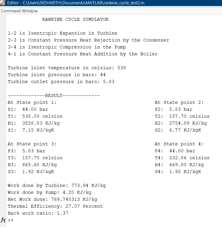
Turbine inlet temperature `= 538^@ C`

Turbine inlet pressure `= 44` bar

Turbine outlet pressure `= 5.83` bar

All the state points and calculations are computed based on the user inputs.

Output shown on the command window,

T-s diagram of the ideal Rankine cycle,

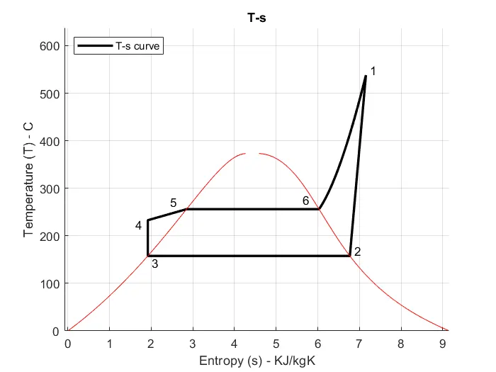
The red curve represents the phase of water in the system, left from the bell-shaped curve is saturated liquid, right from it is saturated vapour, and under the curve is saturated liquid-vapour equilibrium.

h-s diagram of the ideal rankine cycle,

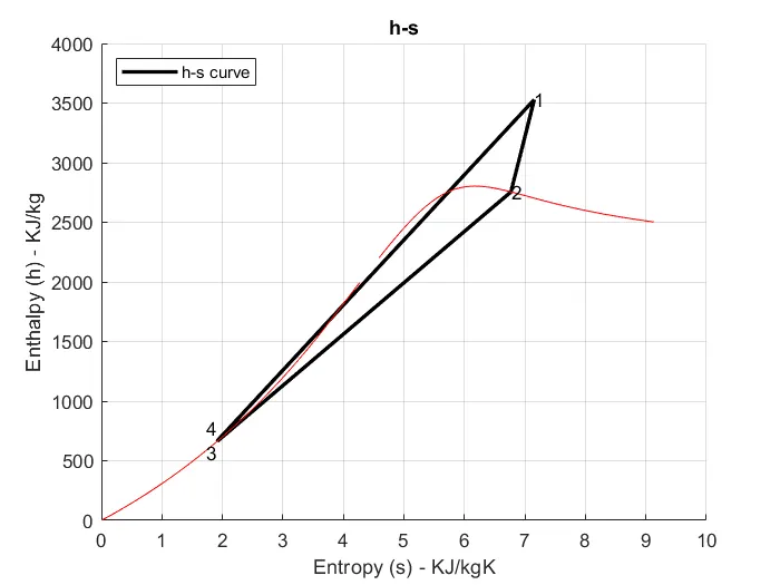
Calculations obtained from the given input,

Net Output work = 769.740313 KJ/kg

Thermal Efficiency = 27.07%

Back work ratio = 1.37