Parsing NASA thermodynamic data
Aim: To read the NASA Thermodynamic data file and to extract the 14 coefficients of all the species inorder to calculate their specific heat (`C_p`), enthalpy (`H`) and entropy (`S`).
Theory: The data file consist of a list of 53 species along with their 14 coefficients and their local temperature ranges. The coefficients can be represented by a1, a2, a3.... a12, a13, a14. The first 7 coefficients represent the High Temperature coefficients while the rest 7 coefficients represents the Low Temperature coefficients.
The equation to calculate `C_p`, `H` & `S` is as follows,
`C_p/R = a1 + a2 T + a3 T^2 + a4 T^3 + a5 T^4`
`H/(RT) = a1 + (a2 T)/2 + (a3 T^2)/3 + (a4 T^3)/4 + (a5 T^4)/5 + (a6)/T`
`S/R = a1 lnT + a2 T + (a3 T^2)/2 + (a4 T^3)/3 + (a5 T^4)/4 + a7`
Here R is the universal gas constant whose value is `8.314 J mol^-1 K^-1`, and T is the temperature with in the local temperature range. So different value of `C_p`, `H` & `S` for each of the species can be obtained by varying T.
The main program code is as follows,
close all
clear all
clc


f1 = fopen('THERMO.dat','r');                   %opens THERMO.dat file for reading, f1 is the file pointer
fgetl(f1);                                      %skips first line
data_line = fgetl(f1);                          %reads next line and stores it into data_line variable
globaltempdata = strsplit(data_line,' ');       %splits the string at the specified delimiter, ' '
global_min_temp = str2num(globaltempdata{2});
global_med_temp = str2num(globaltempdata{3});
global_max_temp = str2num(globaltempdata{4});
R = 8.314;                                      %Universal Gas Constant

%loop to skip the comment line
for i = 1:3
    fgetl(f1);
end

%FOR loop to read each of the 53 species data
for i = 1:53
    data_line = fgetl(f1);
    species_name = data_line(1:6);                      %species name
    tempdata = strsplit(data_line,' ');
    local_min_temp = str2num(tempdata{end-3});          %local minimum temperature
    local_mid_temp = str2num(tempdata{end-1});          %local middle temperature
    local_max_temp = str2num(tempdata{end-2});          %local maximum temperature
    T = linspace(local_min_temp,local_max_temp,1000);   %local temperature range


    %print the molecular weight of each species on the command window
    fprintf('Molecular weight of %s = %f g/mole n',species_name,molecular_mass_cal(species_name))


    %reading the second line of each species
    data_line = fgetl(f1);
    epos = strfind(data_line,'E'); %find the letters 'E' in the string

    %coefficient 1
    a1 = data_line(epos(1)-11:epos(1)-1);
    a1 = str2double(a1);                    %convert string to double precision values
    %power of 10 for coefficient 1
    e1 = data_line(epos(1)+1:epos(2)-12);
    e1 = str2double(e1);

    %coefficient 2
    a2 = data_line(epos(2)-11:epos(2)-1);
    a2 = str2double(a2);
    %power of 10 for coefficient 2
    e2 = data_line(epos(2)+1:epos(3)-12);
    e2 = str2double(e2);

    %coefficient 3
    a3 = data_line(epos(3)-11:epos(3)-1);
    a3 = str2double(a3);
    %power of 10 for coefficient 3
    e3 = data_line(epos(3)+1:epos(4)-12);
    e3 = str2double(e3);

    %coefficient 4
    a4 = data_line(epos(4)-11:epos(4)-1);
    a4 = str2double(a4);
    %power of 10 for coefficient 4
    e4 = data_line(epos(4)+1:epos(5)-12);
    e4 = str2double(e4);

    %coefficient 5
    a5 = data_line(epos(5)-11:epos(5)-1);
    a5 = str2double(a5);
    %power of 10 for coefficient 5
    e5 = data_line(epos(5)+1:epos(5)+4);
    e5 = str2double(e5);

    %reading the third line of each species
    data_line = fgetl(f1);
    epos = strfind(data_line,'E');

    %coefficient 6
    a6 = data_line(epos(1)-11:epos(1)-1);
    a6 = str2double(a6);
    %power of 10 for coefficient 6
    e6 = data_line(epos(1)+1:epos(2)-12);
    e6 = str2double(e6);

    %coefficient 7
    a7 = data_line(epos(2)-11:epos(2)-1);
    a7 = str2double(a7);
    %power of 10 for coefficient 7
    e7 = data_line(epos(2)+1:epos(3)-12);
    e7 = str2double(e7);

    %coefficient 8
    a8 = data_line(epos(3)-11:epos(3)-1);
    a8 = str2double(a8);
    %power of 10 for coefficient 8
    e8 = data_line(epos(3)+1:epos(4)-12);
    e8 = str2double(e8);

    %coefficient 9
    a9 = data_line(epos(4)-11:epos(4)-1);
    a9 = str2double(a9);
    %power of 10 for coefficient 9
    e9 = data_line(epos(4)+1:epos(5)-12);
    e9 = str2double(e9);

    %coefficient 10
    a10 = data_line(epos(5)-11:epos(5)-1);
    a10 = str2double(a10);
    %power of 10 for coefficient 10
    e10 = data_line(epos(5)+1:epos(5)+4);
    e10 = str2double(e10);

    %reading the fourth line of each species
    data_line = fgetl(f1);
    epos = strfind(data_line,'E');

    %coefficient 11
    a11 = data_line(epos(1)-11:epos(1)-1);
    a11 = str2double(a11);
    %power of 10 for coefficient 11
    e11 = data_line(epos(1)+1:epos(2)-12);
    e11 = str2double(e11);

    %coefficient 12
    a12 = data_line(epos(2)-11:epos(2)-1);
    a12 = str2double(a12);
    %power of 10 for coefficient 12
    e12 = data_line(epos(2)+1:epos(3)-12);
    e12 = str2double(e12);

    %coefficient 13
    a13 = data_line(epos(3)-11:epos(3)-1);
    a13 = str2double(a13);
    %power of 10 for coefficient 13
    e13 = data_line(epos(3)+1:epos(4)-12);
    e13 = str2double(e13);

    %coefficient 14
    a14 = data_line(epos(4)-11:epos(4)-1);
    a14 = str2double(a14);
    %power of 10 for coefficient 14
    e14 = data_line(epos(4)+1:epos(4)+4);
    e14 = str2double(e14);

    %FOR loop to calculate Cp, H & S
    for j = 1:length(T)
        %if the temperature is more than the value of the middle
        %temperature then the high temperature equation is used otherwise
        %the low temperature equation is used to do the calculation

        if T(j)>local_mid_temp
            %high temperature equations
            Cp = (a1*10^e1 + a2*10^e2*T + a3*10^e3*T.^2 + a4*10^e4*T.^3 + a5*10^e5*T.^4)*R;
            H = (a1*10^e1 + a2*10^e2*T/2 + a3*10^e3*(T.^2)/3 + a4*10^e4*(T.^3)/4 + a5*10^e5*(T.^4)/5 + (a6*10^e6)./T).*R.*T;
            S = (a1*10^e1*log(T) + a2*10^e2*T + a3*10^e3*(T.^2)/2 + a4*10^e4*(T.^3)/3 + a5*10^e5*(T.^4)/4 + a7*10^e7)*R;
        else
            %low temperature equations
            Cp = (a8*10^e8 + a9*10^e9*T + a10*10^e10*T.^2 + a11*10^e11*T.^3 + a12*10^e12*T.^4)*R;
            H = (a8*10^e8 + a9*10^e9*T/2 + a10*10^e10*(T.^2)/3 + a11*10^e11*(T.^3)/4 + a12*10^e12*(T.^4)/5 + (a13*10^e13)./T).*R.*T;
            S = (a8*10^e8*log(T) + a9*10^e9*T + a10*10^e10*(T.^2)/2 + a11*10^e11*(T.^3)/3 + a12*10^e12*(T.^4)/4 + a14*10^e14)*R;
        end
    end

    %figure 1 stores the plot for specific heat
    figure(1)
    plot(T,Cp,'linewidth',2)
    xlabel('Temperature (K)')
    ylabel('Specific Heat - Cp (J/mol K)')
    title(species_name)
    grid on

    %figure 2 stores the plot for enthalpy
    figure(2)
    plot(T,H,'linewidth',2)
    xlabel('Temperature (K)')
    ylabel('Enthalpy - H (J)')
    title(species_name)
    grid on

    %figure 3 stores the plot for entropy
    figure(3)
    plot(T,S,'linewidth',2)
    xlabel('Temperature (K)')
    ylabel('Entropy - S (J/K)')
    title(species_name)
    grid on

    %To create directory for each of the species inorder to store their
    %respective plots for Cp, H & S
    cd 'C:UsersSIDHARTHDocumentsMATLAB'                    %changes the directory
    if ~exist('NASA_Thermo','dir')                              %checks if the directory 'NASA_Thermo' exists or not
        mkdir('NASA_Thermo')                                    %creates the directory if it does not exist
        cd 'C:UsersSIDHARTHDocumentsMATLABNASA_Thermo'    %changes directory to the created directory
    else
        cd 'C:UsersSIDHARTHDocumentsMATLABNASA_Thermo'    %if directory already exist the folder is opened
    end
    if ~exist(species_name,'dir')                               %checks if the directory in the name of the species exist or not
        mkdir(species_name)                                     %create directory in the name of the species
        directory = (['C:UsersSIDHARTHDocumentsMATLABNASA_Thermo',species_name]);
        cd(directory)
    else
        directory = (['C:UsersSIDHARTHDocumentsMATLABNASA_Thermo',species_name]);
        cd(directory)
    end

    %exports or saves the plot as images
    exportgraphics(figure(1),'Specific Heat - Cp.png','Resolution',600);
    exportgraphics(figure(2),'Enthalpy - H.png','Resolution',600);
    exportgraphics(figure(3),'Entropy - S.png','Resolution',600);

end

%closes the opened file
fclose(f1)
The function code for molecular weight is as follows,
function [molecular_mass] = molecular_mass_cal(species)
wt_sum = 0;
elements = ['C','H','O','N','S','A'];
atomic_wt = [12.011, 1.007, 15.999, 14.006, 32.06, 39.948];

for i = 1:length(species)
    for j = 1:length(elements)
        if strcmp(species(i),elements(j))
            wt_sum = wt_sum + atomic_wt(j);
            flag = j;
        end
    end
    n = str2num(species(i));
    if n >= 1
        wt_sum = wt_sum + atomic_wt(flag)*(n-1);
    end
end
molecular_mass = wt_sum;
end
Code Logic
fopen() command is used to open and read the file THERMO.dat and fgetl() command is used to read each line of the file.
The first 5 lines of the file is not needed to calculate the equation so they can be ignored, fgetl() is used to skip these line.
In order to read the data of all 53 species from the file a FOR loop is needed, the loop is run 53 times. Each species data contains 4 lines the first line gives the name of the species and its local temperature range and the next 3 lines give its coefficients.
Each of the species data appears similar to each other, their format is the same. The species data shown below is that of the oxygen atom,
O                 L 1/90O   1               G   200.000  3500.000  1000.000    1
 2.56942078E+00-8.59741137E-05 4.19484589E-08-1.00177799E-11 1.22833691E-15    2
 2.92175791E+04 4.78433864E+00 3.16826710E+00-3.27931884E-03 6.64306396E-06    3
-6.12806624E-09 2.11265971E-12 2.91222592E+04 2.05193346E+00                   4
Assigning the fgetl to a variable, the character vector of that particular line can be obtained through the assigned variable.
data_line = fgetl(f1);
species_name = data_line(1:6);
The first few characters of the first line of the species data contains the name of the species, using the range function of MatLAB, the name of the species can be retrevied.
tempdata = strsplit(data_line,' ');
local_min_temp = str2num(tempdata{end-3});          %local minimum temperature
local_mid_temp = str2num(tempdata{end-1});          %local middle temperature
local_max_temp = str2num(tempdata{end-2});          %local maximum temperature
T = linspace(local_min_temp,local_max_temp,1000);   %local temperature range
Using the strsplit command with the delimiter set as ' ' (space), the local temperature ranges can be obtained. The strsplit command splits the string at the set delimiter, it returns as cell arrays containing the character vectors. These character vectors cannot be directly used in calculation, so str2num command converts the string or character vectors into numeric array.
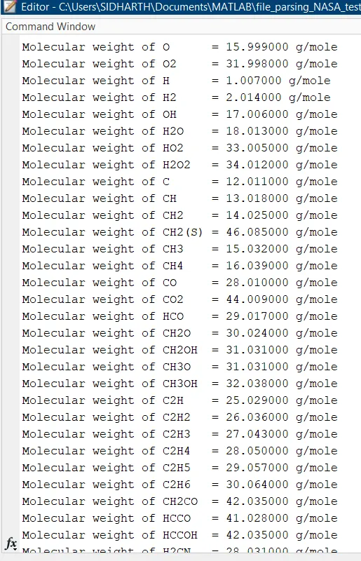
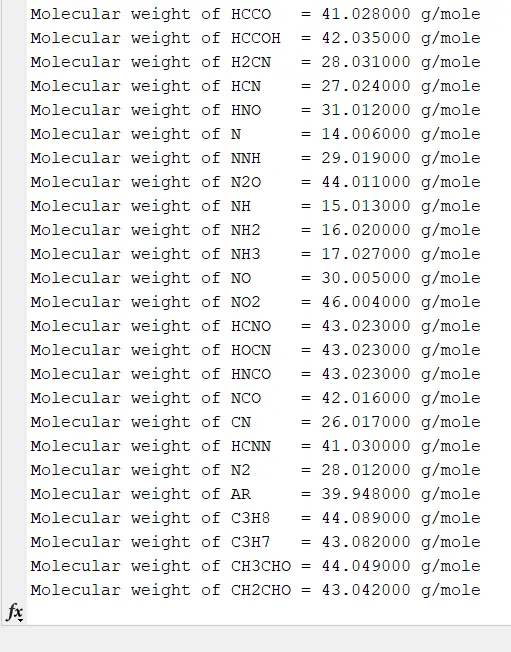
fprintf('Molecular weight of %s = %f g/mole n',species_name,molecular_mass_cal(species_name))This line prints the molecular weight of each species line by line in the command window. Here the molecular weight is calculated and returned by a custom made function called molecular_mass_cal(species_name). The input argument for the function is the name of the species. The function contains 2 arrays, one consisting of all the elements the different species from the data can have and the other consist of the respective elements atomic weight.
elements = ['C','H','O','N','S','A'];
atomic_wt = [12.011, 1.007, 15.999, 14.006, 32.06, 39.948];
for i = 1:length(species)
    for j = 1:length(elements)
        if strcmp(species(i),elements(j))
            wt_sum = wt_sum + atomic_wt(j);
            flag = j;
        end
    end
    n = str2num(species(i));
    if n >= 1
        wt_sum = wt_sum + atomic_wt(flag)*(n-1);
    end
end
The function also contains a nested FOR loop which compares each character of the species_name to the element array, the inner loop controls the array of the elements and the outer loop controls the characters of the species name, the strcmp command is used for this purpose. If the comparison returns true then the weight of the element is added to the sum, which is assigned 0 at the start of the function. After the inner loop ends, the character array of the string is converted to numeric array and checked if its value is greater than or equal to 1, if the condition returns true then the weight of the last element that returned true during strcmp will be added to the sum or if the condition returns false the outer FOR loop repeats till the loop ends. After the end of the loop the function returns the sum as the molecular weight.
The next 3 lines of each species contains the coefficient data, there are 5 coefficients in the `2^(nd)` and `3^(rd)` line and 4 coefficients in the `4^(th)` line of each species data. The coefficients are all expressed in scientific notations with the exponent of 10. The logic here is to identify the location of the exponent of 10 then read the decimal fractions and the power of 10.
epos = strfind(data_line,'E');The strfind(string,pattern) command is used to find the letter E within each data_line, this command returns an array that gives the vector positions of the letter E within the string.
a1 = data_line(epos(1)-11:epos(1)-1);
a1 = str2double(a1);
e1 = data_line(epos(1)+1:epos(2)-12);
e1 = str2double(e1);
Shown above is how the values for the first coefficient is retrieved, the colon operator is used. str2double converts the string into a double precision. Here a1 gives the decimal fraction while e1 gives the power of 10. The following equation gives the correct value of the coefficient 1.
coefficient_1 = a1*10^e1This is how coefficient 1 is represented. Similarly each of the coefficients can be easily calculated.
In order to calculate `C_p`, `H` and `S` there are 2 sets of equations for each, one using high temperature coefficients and the other using low temperature coefficients. FOR loop is used to do the calculation for each value in the temperature range. The temperature range is divided into 1000 equally spaced points. The local middle temperature (respresented by local_mid_temp) is the dividing point between the high and low temperature section in the temperature range. if-else command is used to do the calculations using the high and low temperature coefficients. If the temperature is more than the value of local middle temperature then the high temperature coefficient is used otherwise the low temperature coefficient is used to do the calculation.
for j = 1:length(T)
    if T(j)>local_mid_temp
        %high temperature equations
        Cp = (a1*10^e1 + a2*10^e2*T + a3*10^e3*T.^2 + a4*10^e4*T.^3 + a5*10^e5*T.^4)*R;
        H = (a1*10^e1 + a2*10^e2*T/2 + a3*10^e3*(T.^2)/3 + a4*10^e4*(T.^3)/4 + a5*10^e5*(T.^4)/5 + (a6*10^e6)./T).*R.*T;
        S = (a1*10^e1*log(T) + a2*10^e2*T + a3*10^e3*(T.^2)/2 + a4*10^e4*(T.^3)/3 + a5*10^e5*(T.^4)/4 + a7*10^e7)*R;
    else
        %low temperature equations
        Cp = (a8*10^e8 + a9*10^e9*T + a10*10^e10*T.^2 + a11*10^e11*T.^3 + a12*10^e12*T.^4)*R;
        H = (a8*10^e8 + a9*10^e9*T/2 + a10*10^e10*(T.^2)/3 + a11*10^e11*(T.^3)/4 + a12*10^e12*(T.^4)/5 + (a13*10^e13)./T).*R.*T;
        S = (a8*10^e8*log(T) + a9*10^e9*T + a10*10^e10*(T.^2)/2 + a11*10^e11*(T.^3)/3 + a12*10^e12*(T.^4)/4 + a14*10^e14)*R;
    end
end
Once the all the calculations are done the next step is to create the plots for `C_p`, `H` and `S`. Seperate figure windows are created for each of the plot using figure(n) command. Once the plots are created, they need to be saved into folders containing the name of the corresponding species. cd command is used to change the current folder to the required location, exist command is then used to check if the folder we are looking for exist or not. If the folder does not exist then mkdir command is used to create a folder with the required name, if the folder already exist then cd is used to navigate into that folder.
cd 'C:UsersSIDHARTHDocumentsMATLAB'
if ~exist('NASA_Thermo','dir')
    mkdir('NASA_Thermo')
    cd 'C:UsersSIDHARTHDocumentsMATLABNASA_Thermo'
else
    cd 'C:UsersSIDHARTHDocumentsMATLABNASA_Thermo'
end
if ~exist(species_name,'dir')
    mkdir(species_name)
    directory = (['C:UsersSIDHARTHDocumentsMATLABNASA_Thermo',species_name]);
    cd(directory)
else
    directory = (['C:UsersSIDHARTHDocumentsMATLABNASA_Thermo',species_name]);
    cd(directory)
end
Once the navigation part is done, the next step is to save the plots created, for this purpose saveas(figure, filename, formattype) command can be used to save the figure to the specific file format but the downside is that the file can only be saved at a resolution of 150 DPI which is does not yield a great result. The other option is to use the exportgraphics(obj, filename, Name, Value) command to save the plot, this command lets the use of additional options like resolution and few others.
exportgraphics(figure(1),'Specific Heat - Cp.png','Resolution',600);
exportgraphics(figure(2),'Enthalpy - H.png','Resolution',600);
exportgraphics(figure(3),'Entropy - S.png','Resolution',600);
This saves the plot under the respective filename at a resolution of 600 DPI.
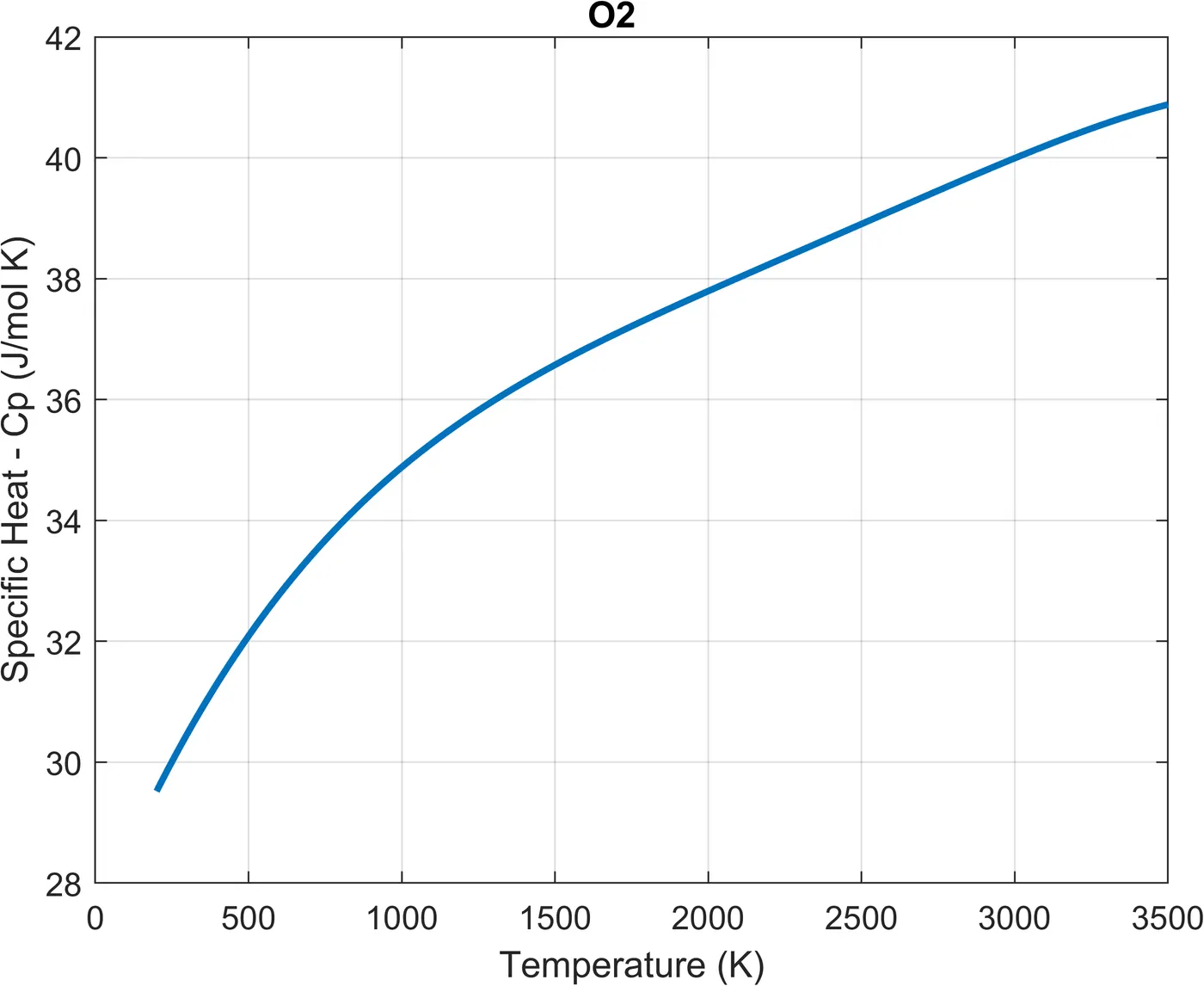
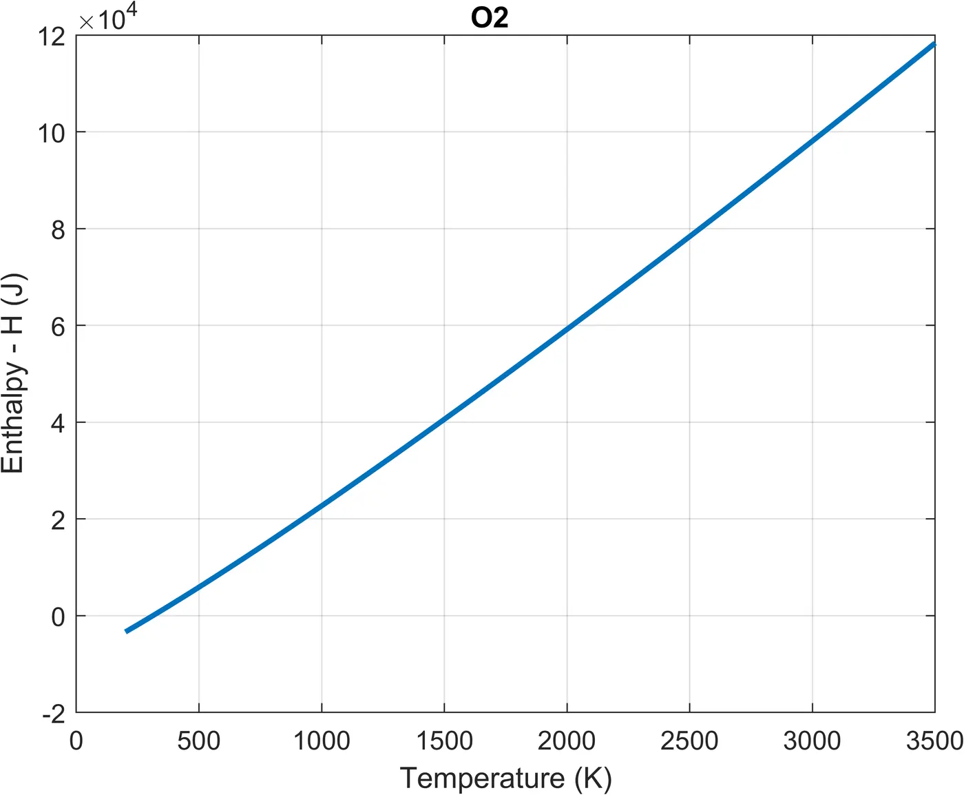
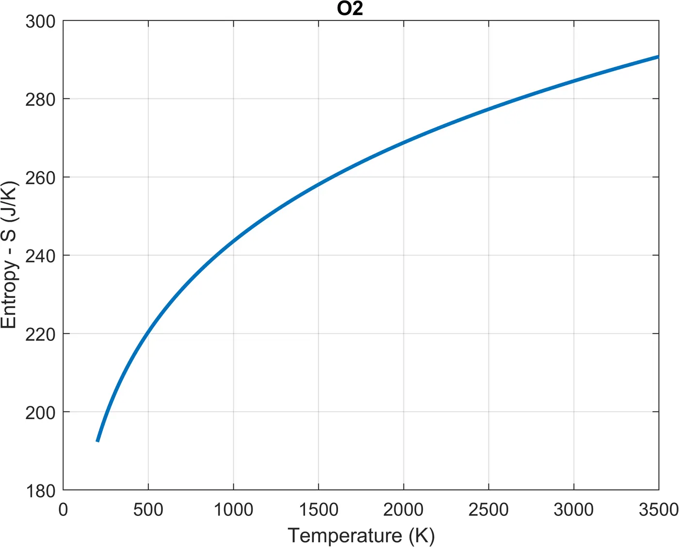
Plots of `O_2`
Specific heat v/s Temperature
Enthalpy v/s Temperature
Entropy v/s Temperature
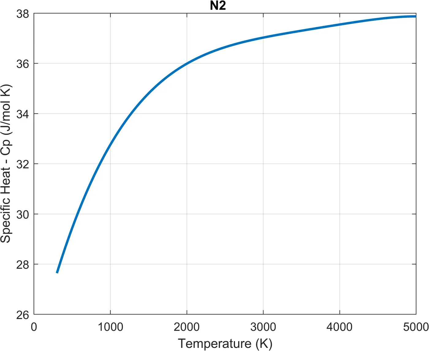
Plots of `N_2`
Specific heat v/s Temperature
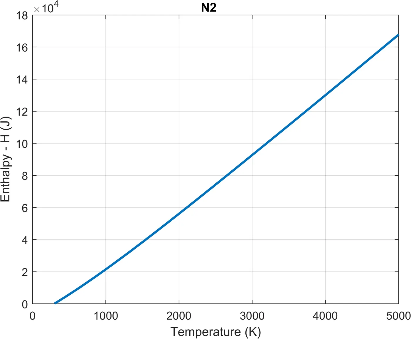
Enthalpy v/s Temperature
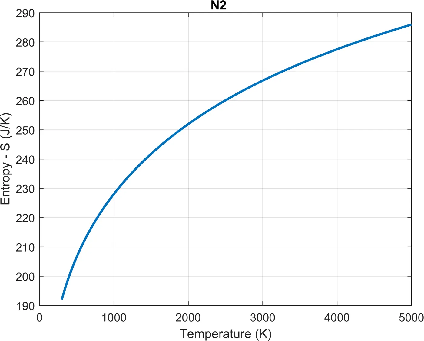
Entropy v/s Temperature
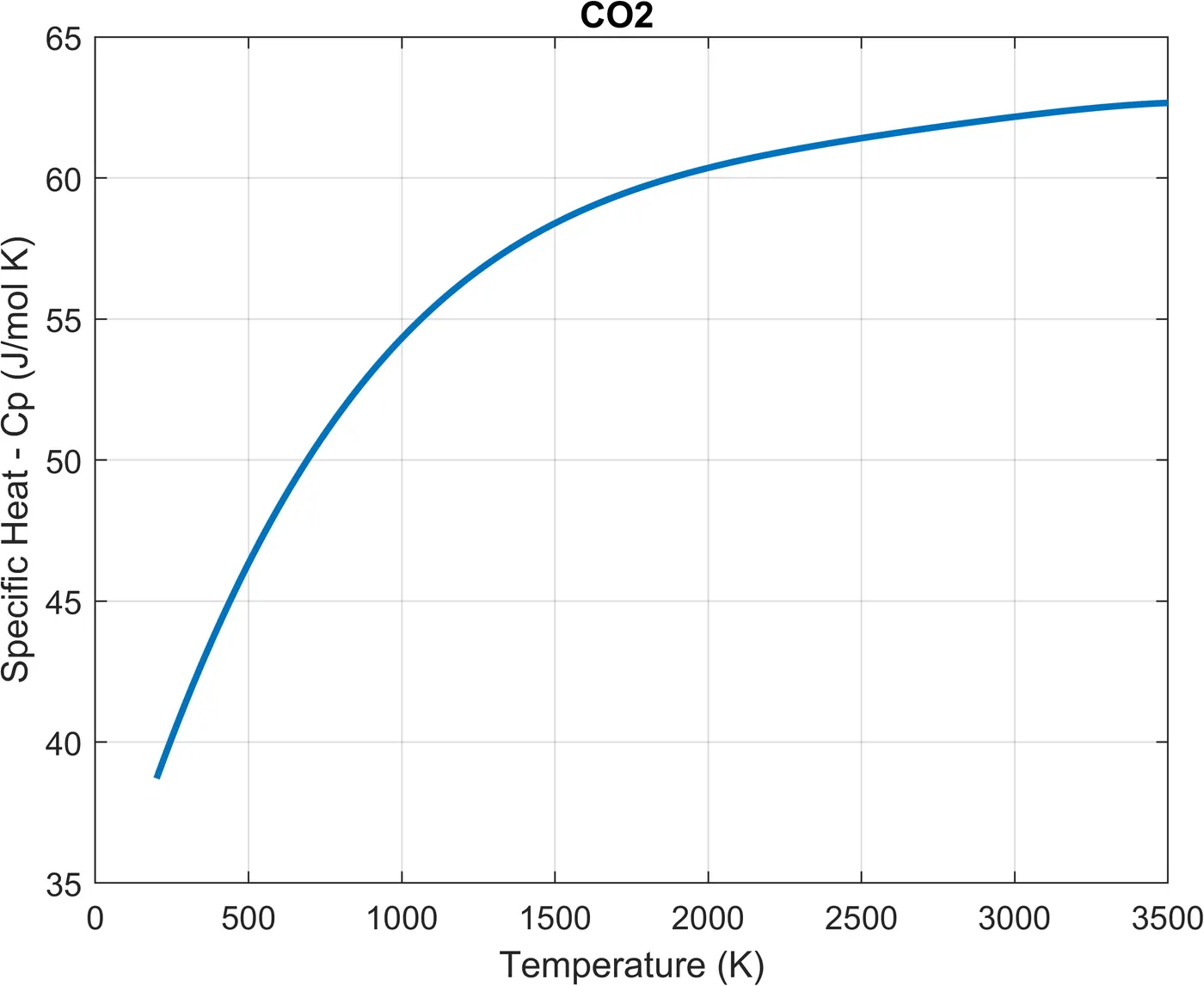
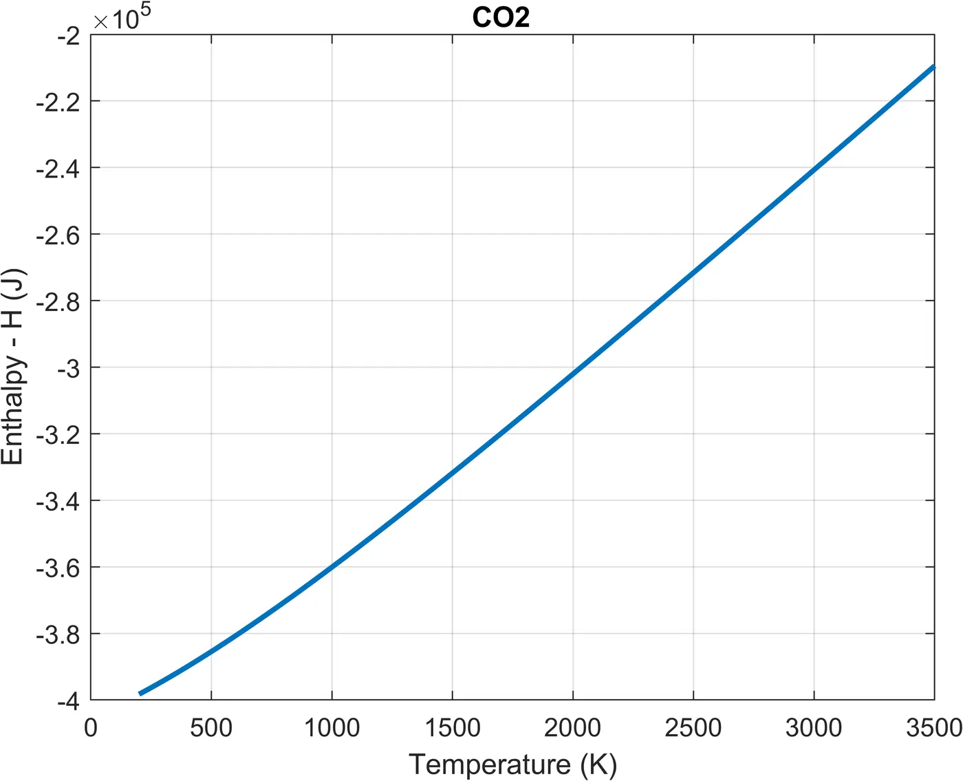
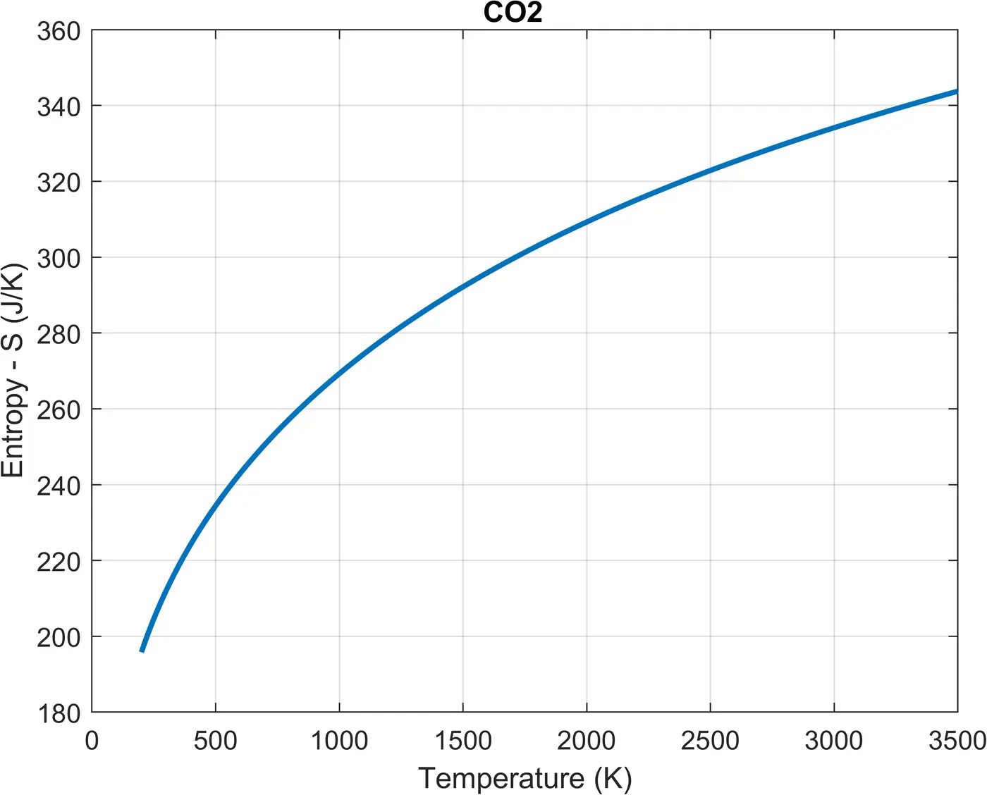
Plots of `CO_2`
Specific heat v/s Temperature
Enthalpy v/s Temperature
Entropy v/s Temperature
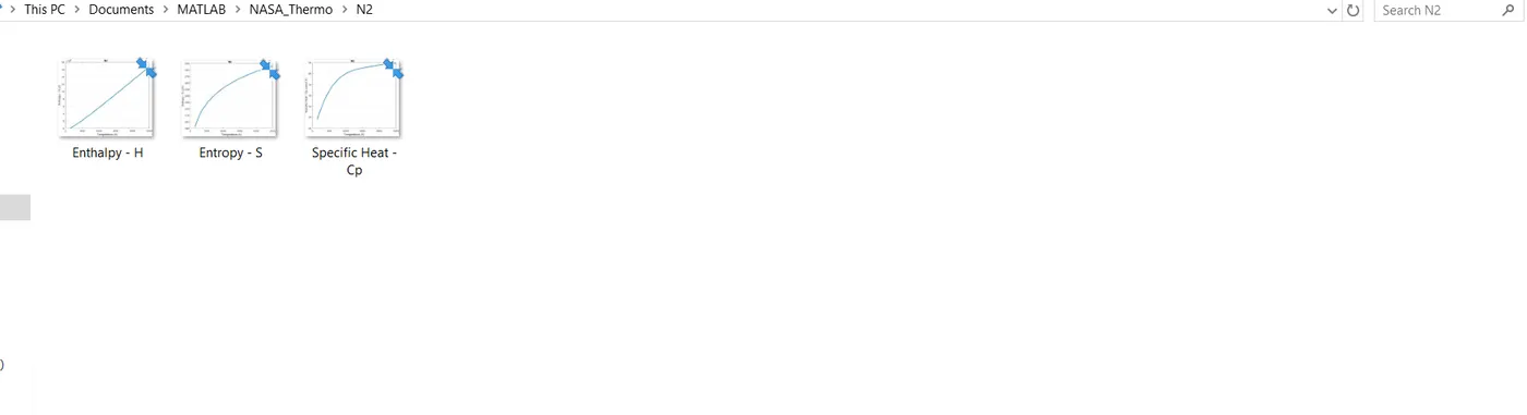
Screenshot of the window containing all the species folder,
Species folder of `N_2` containing the 3 plots,
Molecular Weight of all 53 species shown on the command window,