Week 10 - Simulation of Flow through a pipe in OpenFoam
Aim: The project aims to simulate an axisymmetric flow by applying a wedge boundary condition and validate the following
- Hydrodynamic length with numerical results
- fully developed flow profile with analytical profile
- maximum velocity and pressure drop across the whole pipe
- shear stress for fully developed flow
TOOLS USED: Openfoam CFD tool
THEORY : The Hagen Poiseuille's law gives a measure of pressure drop across an incompressible Newtonian Fluid in the laminar regime going through a long cylindrical pipe of uniform cross section.
Consider the figure below
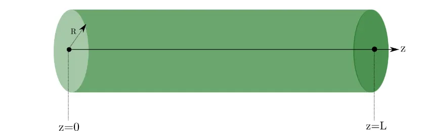
We have a cylindrical pipe with a uniform cross section . Considering the flow is laminar, the formula for pressure drop is given by :
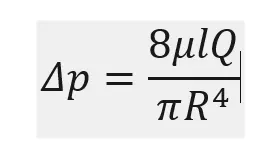
Where delta P is the pressure drop
L is the length of pipe
mu is the dynamic viscosity
Q is the volumetric flow rate
R is the radius of the pipe.
The figure below show how the pressure is distributed along the pipe :
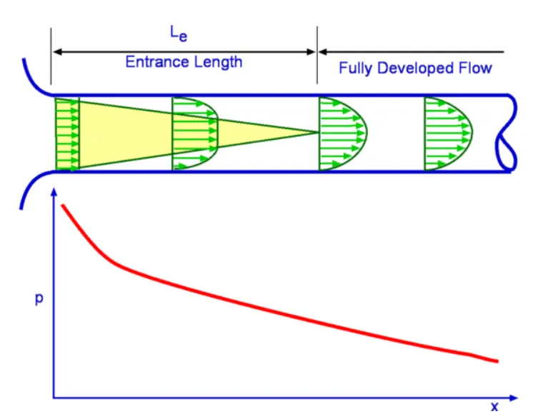
In the entrance region, the fluid is deccelerating , a balance is achieved with inertia, pressure and viscous forces.
ENTRANCE LENGTH OR HYDRODYNAMIC ENTRANCE LENGTH
The entrance length in general defines the the region from the entrance of the pipe where the flow becomes fully developed or it can also be defined as the area following the pipe entrance where effects originating the interior walls of the pipe propagate into the flow as an expanding boundary layer. when the boundary layer expands to fill the entire pipe, the developing flow becomes a fully developed flow. Many kinds of entrance length exists like thermal entrance length, hydrodynamics entrance length but out main focus will be hydrodynamic entrance length.
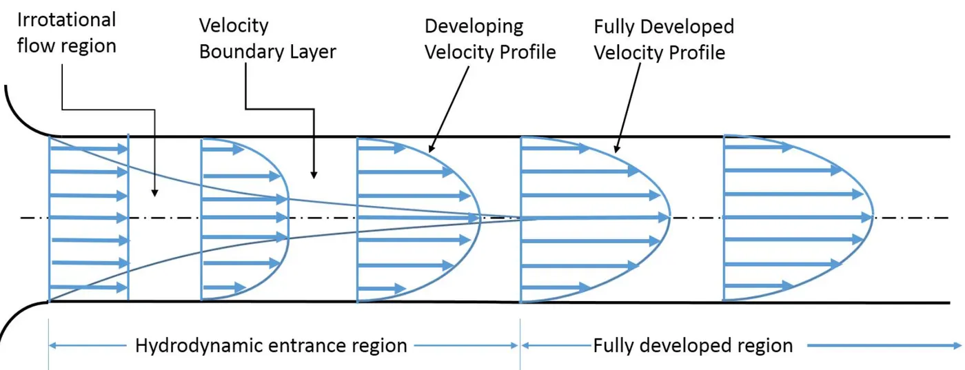
In this particular figure above, it can be seen how the flow is proceeding to the fully developed region. The flow enters with a uniform velocity. Since it is a viscous flow, the walls of the pipe causes the immediate layer to a complete stop(no slip condition) . This further prevents the flow of the layers above as the flow is viscous. This eventually forms a velocity profile. Due to conservation of mass, the velocity will be very high for fluid regions in the center as the flow near the walls is very low. This cause a velocity gradient. After a certain time, the flow becomes fully developed and it does not change.
Boundary Layer :
The layer in which the viscous forces are significant is the boundary layer. It divides the pipe into two regions:
- boundary layer region : The region in which the viscous effects and the velocity changes are significant.
- irrotational flow region : The region in which the viscosity and the velocity changes are insignificant , also known as the inviscid core.
When the fluid enters the pipe, the boundary layers thickness starts to increase from 0 , in the direction of motion of fluid. This eventually reaches the pipe centre and fills the entire pipe. This region from the entrance of the pipe till the point where the boundary layer covers the entire pipe is called as the hydrodynamic region of the pipe and the distance is called the hydrodynamics entrance length. The velocity profile develops in this region and its called hydrodynamically developing flow. After this region, the flow is fully developed and remains unchanged. This is called hydrodynamically fully developed region.
Calculation of hydrodynamic length :
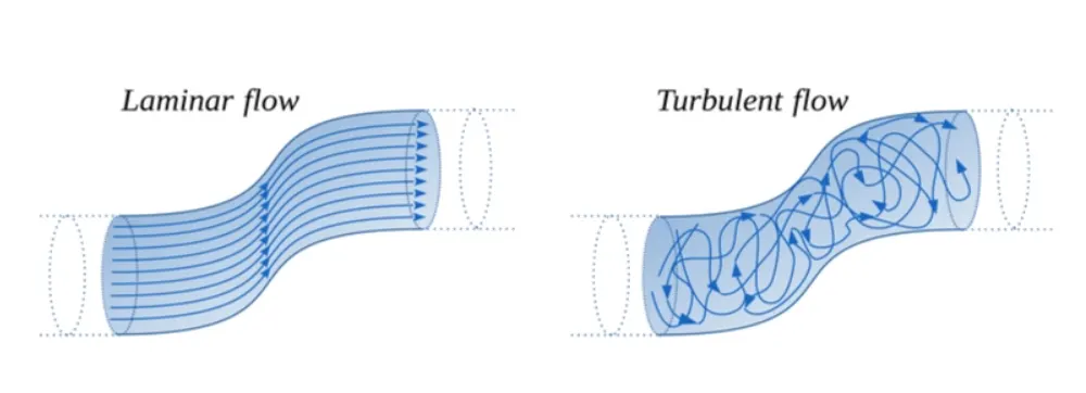
This depends on whether the inlet flow is laminar or turbulent, which is calculated using the Reynolds number given by
Re = rho . V . L / mu
rho = density of the flow : kg/ m^3
V= velocity of the flow : m/s
L= characteristic length : m
mu = dynamic viscosity : kg /(m.s)
AXIS SYMMETRIC BOUNDARY CONDITION:
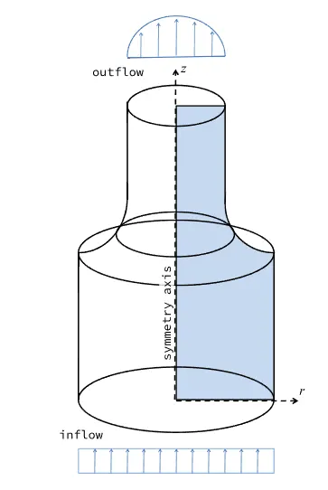
An axisymmetric boundary condition is a boundary condition where the flow variables like pressure and velocity does not change with (theta). Running full 3d simulations can be quite expensive from a computational perspective. So it is always a good practice to simplify the simulations and reduce the dimensions. In an axisymmetric condition , problems that feature cylindrical and rotational symmetric features can be transformed into a 2,5 dimensional problem by doing a cylindrical coordinate transformation. A symmetry axis, usually r=0, is taken as reference around which the coordinates and PDE operators (gradient and divergence) are transformed. In this way the governing equations will be reduced to 2D while representing a rotationally symmetric three dimensional problem.
 bond
bond
Wedge boundary condition :
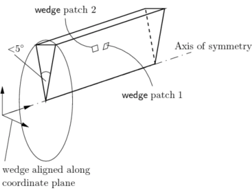
The wedge boundary condition is used to simulate axisymmetric problems
PROPERTY AND ASSUMPTION TABLE :
All properties are calculated at 25 degree celsius
| PROPERTIES | VALUES |
|---|---|
| Length | 2.8 m |
| Density | 997 kg/m3 |
| Dynamic viscosity | 0.89*10^-3 Pas |
| Kinematic Viscosity | .893*10^-6 m^2/s |
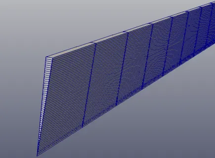
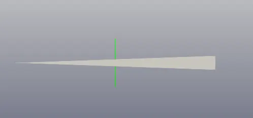
| wedge angle | 4 degree. |
| Diameter | 0.02 |
|---|---|
Calculations :
Given : Re = 2100
Assuming a Diameter of 0.02 m

V = (2100 * 8.9 *10^-4)/(997*0.02)
we get v = 0.0937 m/s
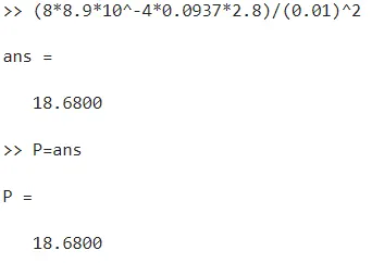
From the Hagen Poiseuille's equation we calculate the pressure drop :
Wedge Geometry :
RESULTS AND DISCUSSION:
1. Validate hydro dynamic length with the numerical result
The code calculates the hydrodynamic entrance length to be 2.4 m . Now from the simulation , we can see that
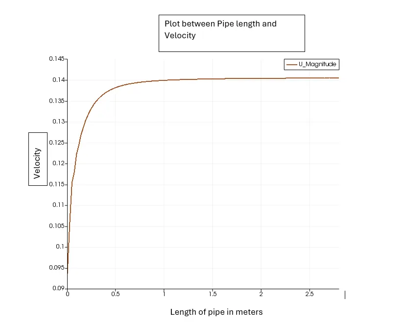
The flow becomes fully developed, at around 2.3-2.4 m in the graph. so the simulation validates the hydrodynamic entrance length.
2. Validate the fully developed flow velocity profile with its analytical profile
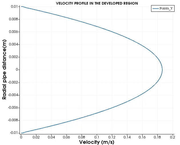
to validate the fully developed velocity profile, we say just need to show if the velocity is changing withing the fully developed region and if this velocity coincides with the calculated values. So the developed region is from 2.4 to 2.8 m, we can select a few values along the x axis and plot them to understand the fully developed region.
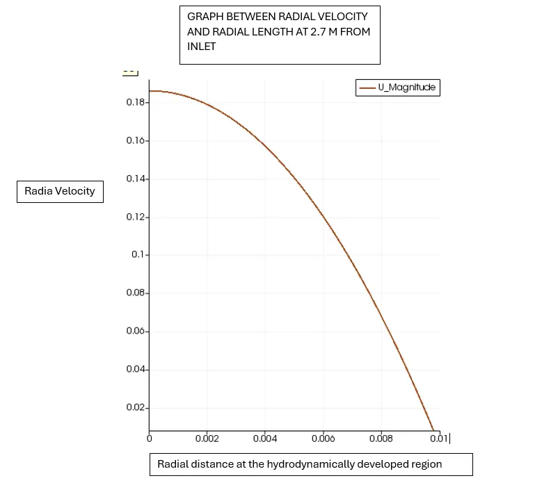
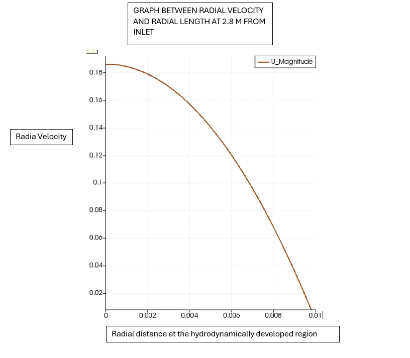
You can see that both the plots are very similar. When mirror imaged , it forms a parabolic profile, which confirms that it is similar to a fully developed flow.
3. Validate maximum velocity and pressure drop for a fully developed flow
The maximum velocity value can be validated using the above graph. It can be seen that the the graph shows a value approximately around 0.185 m/s and the calculated max velocity value is 0.1875 m/s. So it is validated.
to validate the pressure drop we need to we need to setup a plot across the hydrodynamically fully developed region of the pipe , and see how the pressure drop is varying.
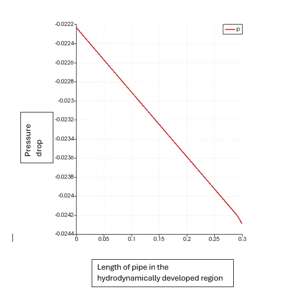
Calculating the pressure drop from the figure, you can see the value comes out to be around : 0.002 pa
from the formula :

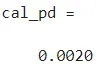
So this is also validated.
4. Post process shear stress and validate wall shear stress for fully developed flow
In the hydrodynamic entrance region, the wall shear stress should be highest at the pipe inlet where the boundary layer thickness is the smallest. Shear stress should decrease along the flow direction .In a fully developed region, the pressure gradient and the shear stress in flow are in balance.
The plot is given below :
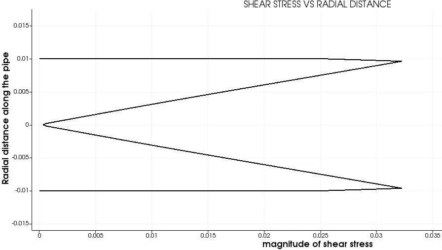
This is the variation of pressure drop along the diameter of the pipe at a distance of 2.5 m from the inlet. This is in the hydrodynamically developed region.
The calculated value from the graph is around 0.033 N/m2. This is the value from the numerical results. Now from the matlab code, the calculated shear stress comes out to be :
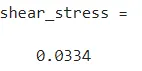
This is the calculated value. It can be seen that both the values are quite similar, so this has been validated.
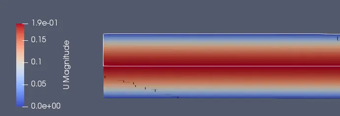
CONTOUR PLOTS
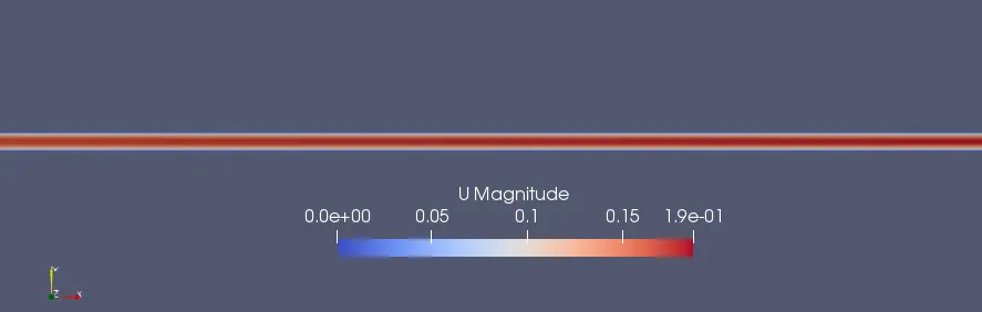
The contour plots below shows the velocity distribution of the flow at the hydrodynamically developed region of the pipe. The reflect option has been used to show the entire pipe diameter.
The pressure distribution can be seen in the contour plots below :
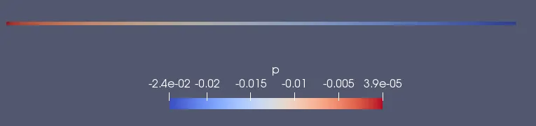
With the same reflect option in ParaFoam, the entire velocity profile has been plotted at the developed region.
CONCLUSION
So here a very detailed study of flow through a pipe has been conducted and certain parameters have been validated. The key learning of this project was to
- Understand Hagen Poiseuillie's Equation and it how it calculates pressure drop for an incompressible laminar flow.
- Understand hydrodynamic entrance length in pipe flow
- Understand the velocity and shear stress profiles in the fully developed region of teh flow.
- Create a blockmeshDict file using matlab.
- Understand post processing in Openfoam.