Week 10 - Simulating Combustion of Natural Gas.

Simulating combustion of natural gas.

OBJECTIVE :

• Perform a combustion simulation on the combustor model and plot the variation of the mass fraction of the different species.
• Add the water content in the fuel from 5% to 30% by mole and observe the effect of it on the results.

Introduction –

Natural gas, colorless highly flammable gaseous hydrocarbon consisting primarily of methane and ethane. Natural gas is one of the major combustion fuels used throughout the globe. Natural gas combustion is an exothermic chemical reaction in which natural gas and oxygen react, producing heat and several chemical byproducts. Byproducts of combustion are a concern, albeit It is certainly cleaner than burning many fossil fuels. To study the combustion of natural gas CFD is used, by simulating combustion mixing of fuel and air, temperature rise, flame propagation, byproduct properties, etc can be predicted. In this study, we will simulate natural gas combustion and find byproduct fractions with the effect of the mixture of water and fuel as inlet, on soot formation.

The constant increase in world energy consumption, that represents a crucial challenge for researchers and scientists. Mostly, fossil fuel undergoes some type of combustion and produces energy and byproducts. Obnoxity of emission is the main concern today because is it raising the global average temperature. Nox is one of the most dangerous byproducts, to limit it, water can be mixed during the combustion of natural gas. In this study, we will study the effect of water quantity at the inlet, on the mass fraction of NOx and soot formation. Combustion is a very complex process because it involves a large number of chemical reactions, which will have multiple steps in their mechanism. CFD software makes this task easy, it provides several models like eddy dissipation, finite rate chemistry, finite rate eddy dissipation model, etc. to find the source of combustion in no time and as a result, it allows you to plot mass fraction plots, contours of temperature and velocity, which is very helpful to visualize flame propagation, hot spot, etc.

Flames can be divided into two types premixed flame and non-premixed(diffusion) flames. These further divided into laminar and turbulent. in premixed fuel and air mixed homogenously before combustion. In non-premixed fuel and air meet during combustion. When a self-sustainable flame propagates at subsonic velocities then the flame is called laminar flame. Turbulent flame is just opposite to that, most of the combustion device produces turbulent flames. In this study, we are assuming that turbulent flame will rise during natural gas combustion. Also, there is no energy source that incites combustion, Burning is starting by turbulence.

In CFD modeling several combustion models are available –

Eddy dissipation model

The eddy dissipation model is based on the concept that chemical reaction is fast relative to the transport processes in the flow. When reactants mix at the molecular level, they instantaneously form products. The model assumes that the reaction rate may be related directly to the time required to mix reactants at the molecular level. The eddy dissipation model was developed for use in a wide range of turbulent reacting flows covering premixed and diffusion flames. Because of its simplicity and robust performance in predicting turbulent reacting flows, this model has been widely applied in the prediction of industrial flames.

The finite chemistry model

The finite-rate chemistry model allows the computation of reaction rates described by the molecular interaction between the components in the fluid. It can be combined with the eddy dissipation model for flames where chemical reaction rates might be slow compared with the reactant mixing rates. The finite-rate chemistry model is best applied to situations where the chemical time scale is rate-limiting. This model can be used in conjunction with both laminar and turbulent flow.

The flamelet model

The flamelet model can provide information on minor species and radicals, such as CO and OH, and accounts for turbulent fluctuations in temperature and local extinction at high scalar dissipation rates, for the cost of solving only two transport equations. The model is only applicable for two-feed systems and requires a chemistry library as input. The model can be used only for non-premixed systems.

Burning velocity model and the extended coherent flame model –

The burning velocity model (BVM) and the extended coherent flame model (ECFM) model the propagation of a premixed or partially premixed flame by solving a scalar transport equation for the reaction progress. The BVM uses an algebraic correlation for modelling the turbulent burning velocity. When using the ECFM, the turbulent burning velocity is closed by solving an additional transport equation for the flame surface density.

Natural gas combustion reaction –

This equation will be used to calculate mass fraction and mole fraction species.

5. Procedure –

In this simulation two different cases are studied, case 1 was focusing on species fraction in combustion and case 2 was focusing on the effect of water with fuel as inlet, on soot formation. The following procedure was followed during the simulation –

Geometry –

We created a two-chambered combustor in CAD software and it was brought it into Spaceclaim and converted to a 2D model because solver takes a lot of time to solve the 3D model.

3D model -

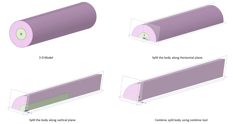
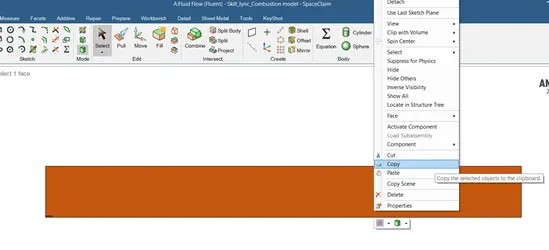
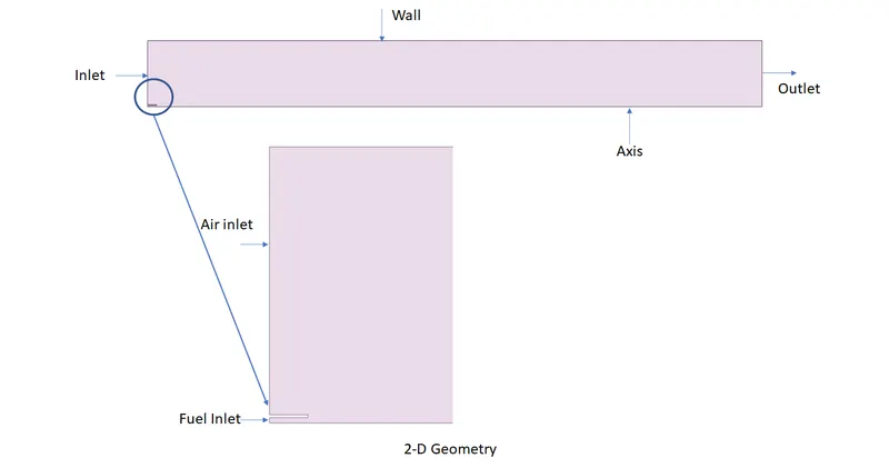
Select the face and copy it to convert the 3D geometry into 2D. There is a slot that is an indication of the separation of fuel and air at the beginning of the combustion process. We chose half of the 2D model because it is symmetric. Simulation results will be the same for both parts.

2D model -

Meshing –

The model was imported from Spaceclaim and tia mesh was deployed with element size 1mm. Named selection was created like fuel inlet, air inlet, wall etc, these used for boundary conditions in solver setup.

Mesh parameters -

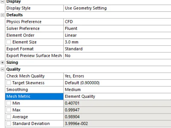
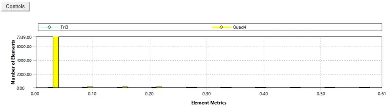
Skewness

Solver setup –

Started with the general setting we proceeded with a pressure-based steady-state solver because fluid flow velocity is very low. In 2D space axisymmetric was chosen due to symmetricity.

General Setting -

Realizable k-epsilon with standard wall functions chosen as solver model, for this simulation flow near the wall was not a major concern. K-omega produces the best result in an analysis of fluid flow near the wall.

Solver Model -

The species model was enabled. Species transport was selected because it solves the conservation equation for all species, which predicts the transport and their production in the combustion zone. In the fluid phase, the volumetric reaction is considered always, so it was selected. Inlet diffusion and diffusion energy source were selected in this setup combustion chamber do not have any ignition source, combustion is arising due to diffusion turbulence of fuel and air. Methane-air-2step selected as mixture material which allows water addition. We proceeded with the eddy dissipation model due to its robustness and it takes less time to solve the model compare to other models.

Species Model -

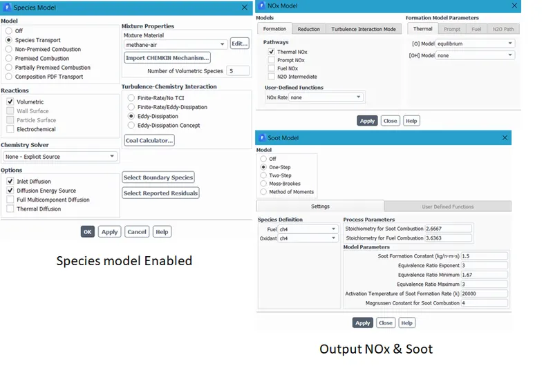
Air inlet velocity was 0.5m/s and fuel inlet velocity were given 80m/s in the boundary condition with 0.23 O2 and 1 CH4 by a mass fraction. These derived from the equation of natural gas combustion.

Total mole fraction OF air = 9.52 moles (2moles O2+2*3.76 moles N2)

Mole fraction of O2 = moles of O2/total moles = 2/9.52 = 0.21

Mass fraction of O2 in air = 0.23

Moles of CH4 = 1

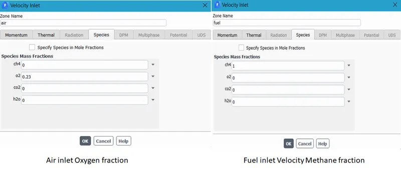
Mole fraction or mass fraction can be given to specify species. Nox model and soot model also enabled because we wanted to analyse Nox and soot formation.

Inlet Boundary conditions -

Air & Fuel inlet -

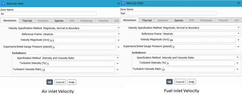
Results –

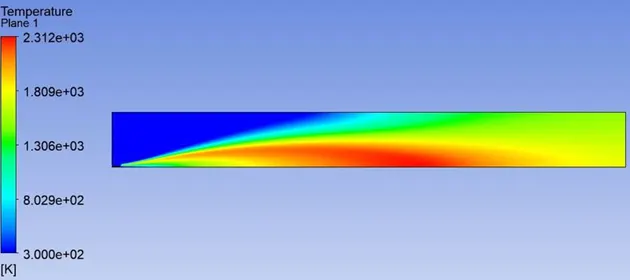
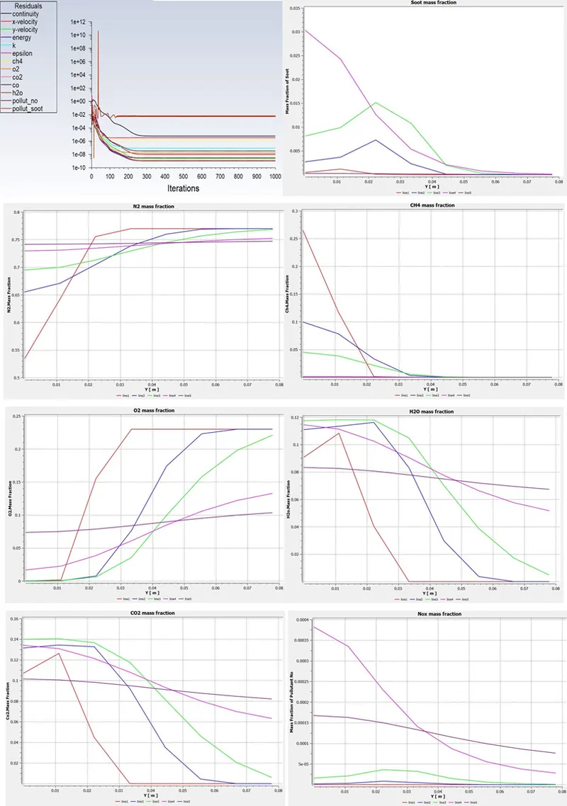
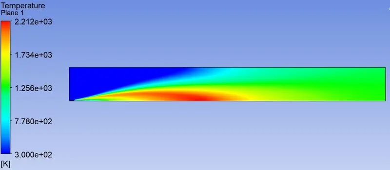
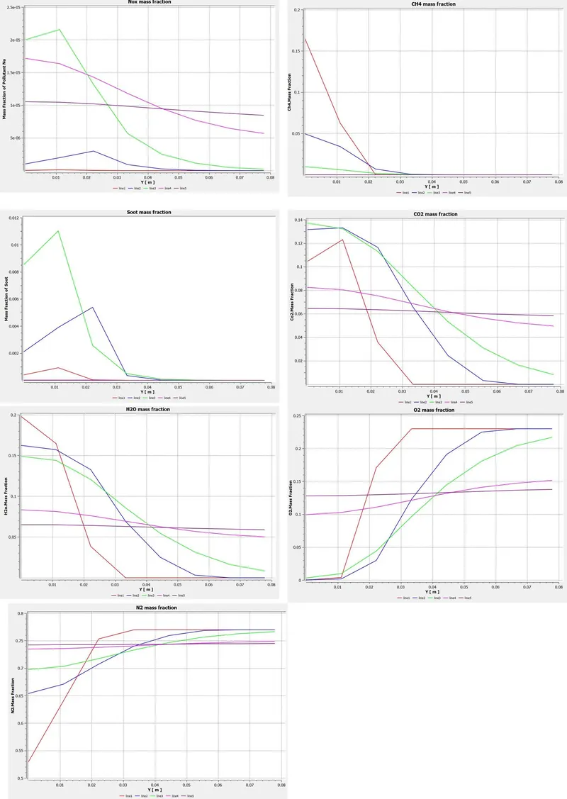
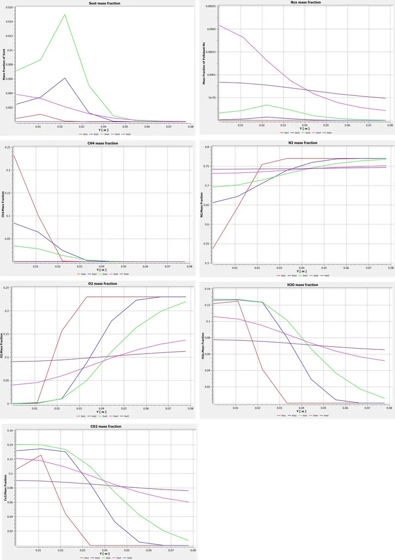
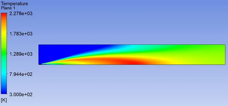
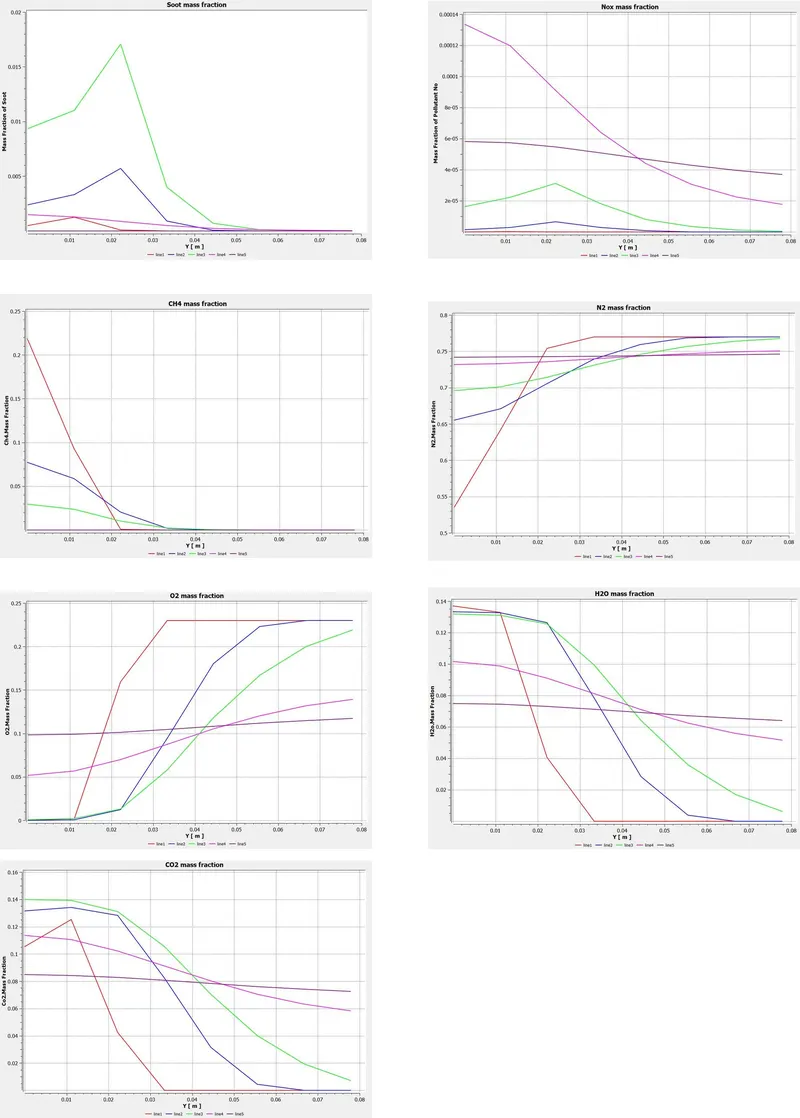
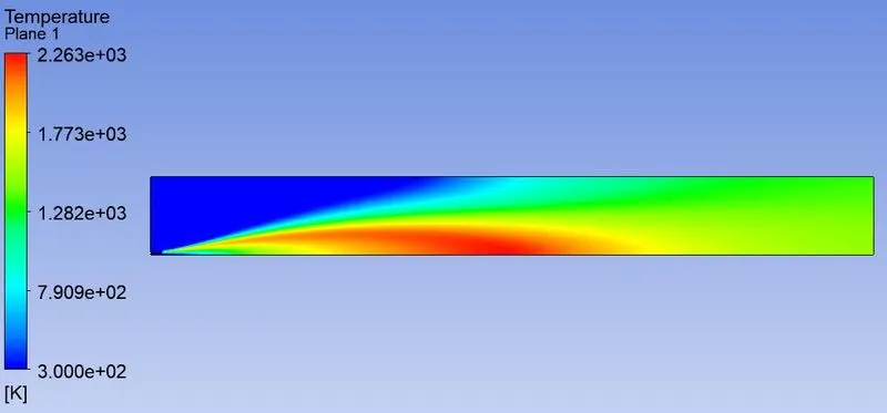
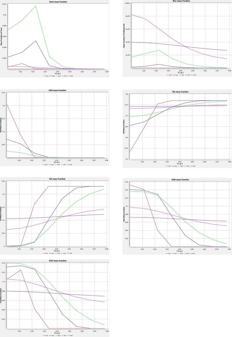
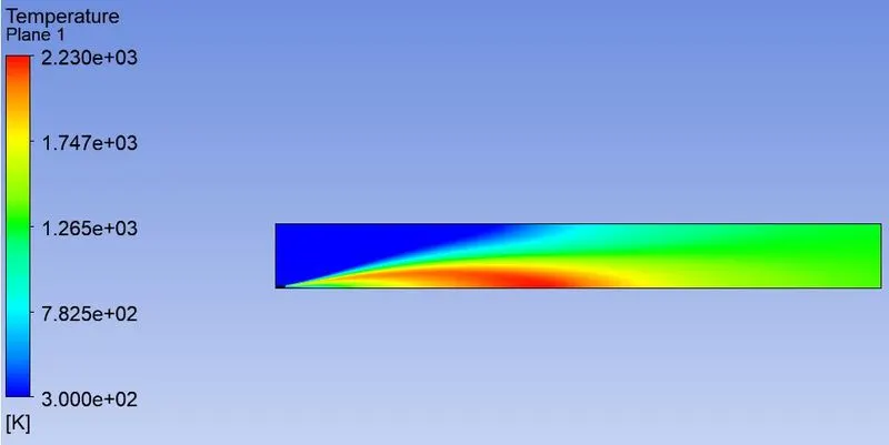
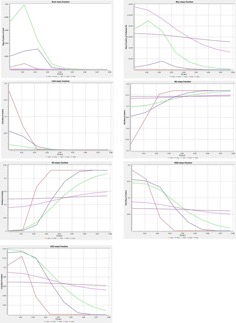
Temperature contour was created to get insights into the flame front and temperature hotspots. Five probe lines were created at distance 0.1x, 0.2x, 0.3x, 0.5x, 0.7x x is the total distance, to inspect the mass fraction of six species CO2, H2O, O2, N2, CH4 and NOx. A chart of soot formation was also plotted. In case 2 fuel is added into the chamber with water from 5% to 30% to investigate the effect of water on soot formation.

Case I

Temperature Contour Plot

Case II

Air-inlet velocity = 0.5m/s, Thermal temperature=300K, Species mixture O2=0.23

Fuel-inlet velocity = 80m/s, Thermal temperature=300K, Species mixture CH4 =1

Temperature Contour Plot

Case III

Adding 5% by mole of water into the fuel mixture

Air-inlet velocity = 0.5m/s, Thermal temperature=300K, Species mixture O2=0.23

Fuel-inlet velocity = 80m/s, Thermal temperature=300K, Species mixture CH4 =0.95,H2O=0.5

Temperature Contour Plot

Case IV

Adding 15% by mole of water into the fuel mixture

Air-inlet velocity = 0.5m/s, Thermal temperature=300K, Species mixture O2=0.23

Fuel-inlet velocity = 80m/s, Thermal temperature=300K, Species mixture CH4 =0.85,H2O=0.15

Temperature Contour Plot

Case V

Adding 25% by mole of water into the fuel mixture

Air-inlet velocity = 0.5m/s, Thermal temperature=300K, Species mixture O2=0.23

Fuel-inlet velocity = 80m/s, Thermal temperature=300K, Species mixture CH4 =0.75,H20=0.25

Temperature Contour Plot

Case VI

Adding 30% by mole of water into the fuel mixture

Air-inlet velocity = 0.5m/s, Thermal temperature=300K, Species mixture O2=0.23

Fuel-inlet velocity = 80m/s, Thermal temperature=300K, Species mixture CH4 =0.7,H2O=0.3

Temperature Contour Plot

Observation

Air inlet Species O2	Fuel Inlet Species	Water Content in fuel	Temperature (K)	Nox	Soot Formation
0.23	1	0	1607	0.00014	4.87E-05
	0.95	0.5	1558	0.0001	1.57E-05
	0.85	0.15	1455	6.08E-05	2.09E-06
	0.75	0.25	1345	3.07E-05	2.45E-07
	0.7	0.3	1345	2.07E-05	7.71E-08

1. Eddy-dissipation model helps us to model the combustion process via turbulence without the presence of an ignition source.
2. Adding water content in the fuel by 5% to 30% by mole leads to a decrease in temperature, NOx emission, and soot formation.
3. Increase in water, decreases temperature, NOx emission, soot formation, increases in N2, O2.
4. A decrease in soot in presence of H2O determines less leakage of fuel and there will be a complete combustion process.

Conclusion

• Thus the simulation of combustion using Ansys fluent ran successfully.
• From the above result, we can say that the formation of NOx and SOOT is reduced by adding water.