Week 10 - Simulating Combustion of Natural Gas.
AIM:- The project aims to simulate the combustion of natural gas.
OBJECTIVE:- The project objectives are-
- In the first section, we need to perform a combustion simulation on the combustor model and plot the variation of the mass fraction of the different species in the simulation using line probes at different locations of the combustor. We need to plot for CO2, H2O, CH4, N2, O2, NOx emissions & Soot formation.
- As we know the Nox and soot are getting formed at the outlet of the combustor. The such formation has harmful effects on the environment and humans. The stringent government norms also demand the least formation of Nox and soot and to satisfy those requirements, we need to check the effect of adding water to the fuel. In this second section, we need to add the water content in the fuel from 5% to 30% per mole and observe the effect of it on the results. It is necessary to provide line plots and contours to prove your claim.
Introduction:-
First, we have to know about the combustion and combustion of natural gas. So, combustion is a chemical process in which a substance reacts rapidly with oxygen and gives out heat and natural gas is one of the major combustion fuels used throughout the country. It is mainly used to generate industrial and utility electric power, produce industrial process steam, and heat residential and commercial spaces. Natural gas consists of a high percentage of methane and varying amounts of ethane, propane, butane, and inerts (typically nitrogen, carbon dioxide, and helium). The average gross heating value of natural gas is approximately 1,050 British thermal units per standard cubic foot (Btu/scf), usually varying from 950 to 1,050 Btu/scf.
Together with the very fast development of civilization, energy demand changed its character and increased. To transform energy, combustion engines are used most often. Their operation, in turn, results in air pollution by toxic substances included in the exhaust gas. The emission of particulate matter, or soot, can be considered a side effect associated with combustion processes characterized by high temperatures and rich conditions. The production of these carbon nanoparticles entails a reduction in the efficiency of the combustion devices, as well as a detrimental effect on climate change and human health.
NOx represents a family of seven compounds. EPA regulates only nitrogen dioxide (NO2 ) as a surrogate for this family of compounds because it is the most prevalent form of NOx in the atmosphere that is generated by anthropogenic (human) activities. NO2 is not only an important air pollutant by itself but also reacts in the atmosphere to form ozone (O3 ) and acid rain.
NOx formed in the high-temperature flame zone near the burners. The formation of NOx is affected by three furnace-zone factors: (1) oxygen concentration, (2) peak temperature, and (3) time of exposure at peak temperature. As these three factors increase, NOx emission levels increase. The emission trends due to changes in these factors are fairly consistent for all types of natural gas-fired boilers and furnaces.
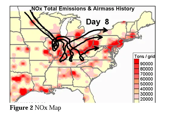
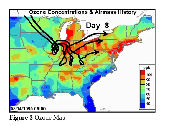
The animated version of Figure 1 shows the trajectory of NOx emissions moving with the weather over 8 days. Figure 2 is a map of ozone concentration that shows the same trajectory over 8 days.
And Soot refers to carbonaceous particles formed during incomplete combustion or pyrolysis of hydrocarbons, including incipient soot particles, mature soot particles, and all of the intermediate particulate stages between inception, maturity, and complete oxidation to gas-phase species.
Therefore, a drastic reduction in emissions is mandatory, demanding a deeper understanding of the formation process, which is still an open issue in combustion chemistry research.
To reduce the amount of NOx emissions from any burner or combustion chamber, water or steam can be injected during normal operation to reduce the temperature of the hot air-fuel mixture. In this project, our work is to simulate the combustion of natural gas and track the emission of NOx and soot formation by plotting the chart then we need to decrease the emission by adding water to the fuel and after that, we also track by adding 5 to 30 % of water with CH4 how much the emission decreases.
Project Description:- Now, first, we will discuss some necessary terms for our simulation. Chemical kinetic modeling is an important tool in the analysis of many combustion systems. It is the branch of physical chemistry that is concerned with understanding the rates of chemical reaction. Chemical kinetics tells us the speed at which chemical species transform into new substances by breaking and reforming their molecular bonds. In other words, it studies the rates and processes of chemical reactions. Chemical kinetic reaction mechanisms are strongly hierarchical in that mechanisms for the combustion of more complex fuels contain within them sub-mechanisms for simpler fuel molecules.
To understand how this chemistry can optimize products, let’s look at a real-world example such as reducing engine emissions. The conversion of fuel into carbon dioxide, water, and various particles powers everyday life. However, the greenhouse and health effects of the end products can’t be ignored. Through the use of chemical kinetics and thermodynamics, engineers can control how the fuel burns to reduce the release of certain pollutants.
We can perform various types of combustion simulations in Ansys Fluent.
Possible type of combustion simulation:-
- Based on Mixing:-
- Non-Premixed Combustion – In the non-premixed flame, fuel and oxidizer are injected into the combustion chamber separately. The reaction rate is mainly controlled by the rate of mixing of fuel and oxidizer, and therefore, the generated flame due to this process is also called diffusion flame.
- Premixed Combustion – Premixed combustion consists of the chemical reactions within a flow of a premixture of reacting species. These reactions occur in a fluid in motion such as would occur in a gas turbine combustor.
- Partially Premixed Combustion – Partially premixed combustion is a hybrid combustion of Homogeneous Charge Compression Ignition(HCCI) and Diesel Combustion, which has great potential in reducing fuel consumption. PPC has a longer premixed time than DC but lesser than HCCI. Therefore it is more stratified than HCCI.
- Based on Phase:-
- Fluid Phase(Volumetric Reaction):-
- Wall(Surface Reactions)
- Particles(Surface Reactions)
- Porous Region(Example – After Treatment System)
In our case, we deal with the Non-premixed combustion simulation.
Basics of Combustion Simulation – To solve any CFD simulation we need to solve those equations
- Continuity Equation
- Momentum Equation
- Energy Equation
If the flows are turbulent then we have to take the turbulence model, here we use the K-Epsilon turbulence model because the flows are turbulent here. So, we need to solve those equations also. But in the case of the Combustion model we need to solve another equation called the Species Transport Equation. The equation is shown below-
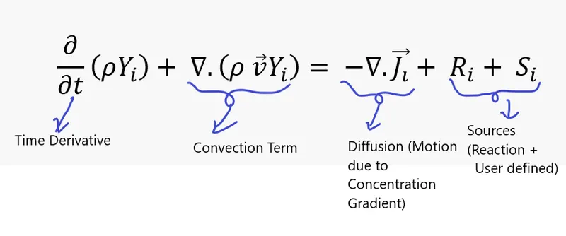
Here, `ρ` is the density of the mixture, Yi is the mass fraction of the particular species and i refers to the species index. In Convection terms, we say that a particular species i moving in our fluid domain based on the current velocity. On the left side, we have the diffusion term and we can understand it with one example. Let’s assume in a particular domain, there is no bulk flow and we have a high concentration of CO2 in a single space and everything else is air. And then CO2 is going to slowly diffuse into the air based upon the gradients in CO2 concentration. And that CO2 diffuses in all directions equally. For engineering simulation, most flows are considered to be turbulent. In that case, our diffusion term is simplified so that it takes into account only the turbulent diffusion. The last two terms are sources. When a chemical reaction takes place new products and new species going to produce.
In that particular case, the reaction equation is –
This is a simple stoichiometric ratio that we need to balance. We get-
- a = 1
- 2b = 4 => b = 2
- 2ar = 2a + b => ar = 2
- 2c = ar * 2*3.76 = 4*3.76 => c = 7.52
So, we have 1 mol of CH4 and this is our fuel. And the air contains 2 mol of oxygen and 7.52 mol of nitrogen and these values we get by balancing the above equation. Therefore,
- The mole fraction of O2 = `2/((2+7.52) )= 2/9.52=0.21`
- The mole fraction of N2 = `7.52/((2+7.52) )= 7.52/9.52=0.79`
Now, we calculate this in the form of a Mass Fraction
- The mass fraction of O2 = `((0.21 ×16))/((0.21 ×16)+(0.79 ×14) ) = 0.23`
- The mass fraction of N2 = `((0.79 ×14))/((0.21 ×16)+(0.79 ×14) ) = 0.77`
So, all the thing which is necessary for our simulation we discussed and now we go for simulation. We divide our simulation into three parts-
- Geometry and Meshing
- Setting Physics
- Postprocessing
Geometry and Meshing:-
This is our 2D geometry where the combustion takes place -

This is how the meshing looks like in our case-
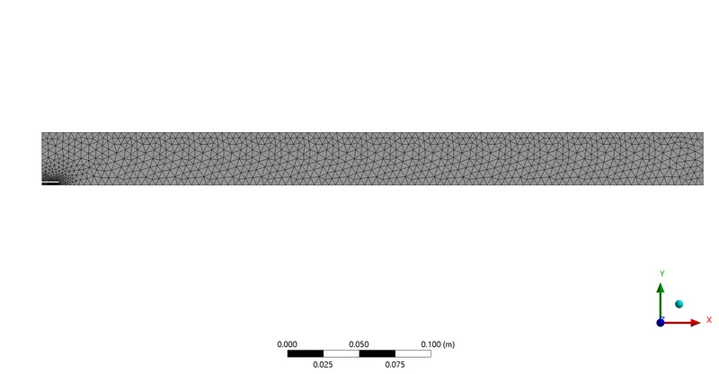
It is the details of our meshing -
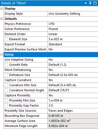

Now we specify the boundery conditions.
Air Inlet:-
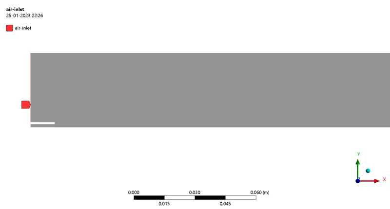
Fuel Inlet:-
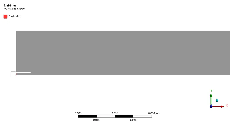
Axis:-
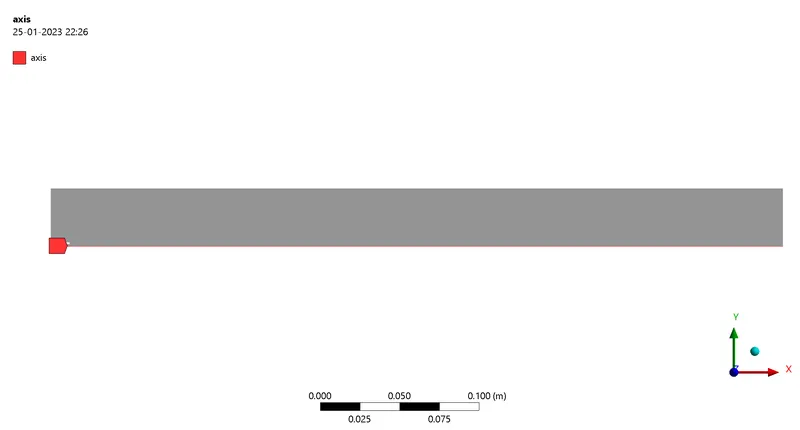
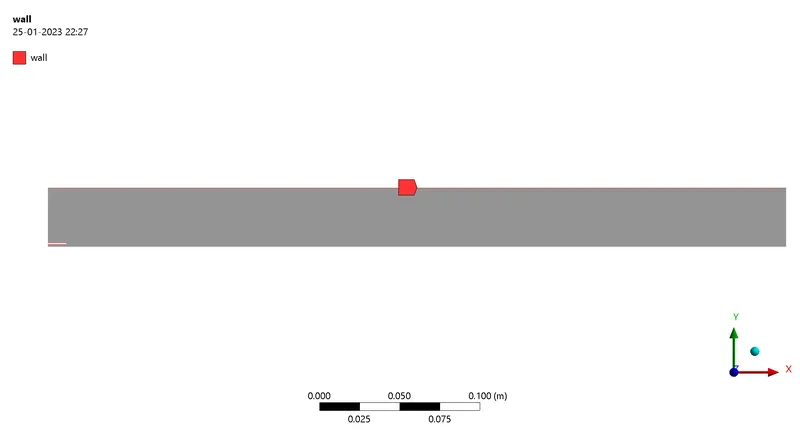
Walls:-
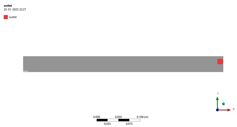
Outlet:-
Setting Physics:-
- Pressure-based solvers and absolute velocity are used.
- It is a 2D Axisymmetric simulation.
- Steady-state simulation is performed.
- The Standard K-epsilon turbulence model is taken as a viscous model. Here, turbulence was modelled by means of the standard k-ε model, which, according to a preliminary analysis, provides the best agreement in terms of mixing.
- Here we take two inlets, one outlet, a wall, and one axis for boundary conditions as we know.
- There are two inlets, one for air and one for fuel. In our case, we only care about the amount of oxygen that comes with air, since when fuel comes into contact with oxygen, combustion occurs. As we discussed in the case of solving our combustion equation, we take 0.23 oxygen. The fuel is CH4, and we add water to it and increase the water amount to 0.3 to reduce NOx emissions and soot formation.
- NOx pollutants and Soot options are enabled to know how much these are produced by this combustion.
- We can see the properties of Reactants and Products below the given report.
- For our case, in burners, the first air and fuel are mixed, and after a certain time combustion takes place that time is calculated by the k-epsilon turbulence model since there is a good amount of turbulence occurs. This is what is called the Turbulence Chemistry Interaction model. So, any model which predicts how the combustion takes place based on the turbulence is called TCI. Now the eddy dissipation model is one such model which uses the k-epsilon turbulence model to calculate a time for reaction. If the K-epsilon is sufficient then combustion takes place even without the ignition source.
- Here we use the Eddy Dissipation model to calculate the rate of production of every species.
- In the burner, we take air velocity as 0.5 m/s and fuel velocity as 80m/s to mix air and fuel properly.
- In pressure velocity coupling, a Coupled scheme is used as we see in the report.
It is a full report for our first simulation without adding water -
Fluent
Version: axi, dp, pbns, spe, ske (axi, double precision, pressure-based,  species, standard k-epsilon)
Release: 22.1.0
Title:


Models
------

   Model                        Settings
   ----------------------------------------------------------------
   Space                        Axisymmetric
   Time                         Steady
   Viscous                      Standard k-epsilon turbulence model
   Wall Treatment               Standard Wall Functions
   Heat Transfer                Enabled
   Solidification and Melting   Disabled
   Radiation                    None
   Species                      Reacting (5 species)
   Coupled Dispersed Phase      Disabled
   NOx Pollutants               Enabled
   SOx Pollutants               Disabled
   Soot                         Enabled
   Mercury Pollutants           Disabled
   Structure                    Disabled
   Acoustics                    Disabled
   Eulerian Wall Film           Disabled
   Potential/Li-ion Battery     Disabled
   Multiphase                   Disabled


Material Properties
-------------------

   Material: methane-air (mixture)

      Property               Units      Method                     Value(s)
      ----------------------------------------------------------------------------------------------------------------------------------------------------------------------------------------------------------------------------------------------------------------------------------------------------------------------
      Mixture Species                   names                      (ch4 o2 co2 h2o n2)
      Reaction                          eddy-dissipation           ((reaction-1 ((ch4 1 0.2 1) (o2 2 1.3 1)) ((co2 1 0 1) (h2o 2 0 1)) ((n2 0 1)) (stoichiometry 1ch4 + 2o2 --> 1co2 + 2h2o) (arrhenius 2.119e+11 2.027e+08 0) (mixing-rate 4 0.5) (specified-rate-exponents? . #t) (use-third-body-efficiencies? . #f)))
      Mechanism                         reaction-mechs             ((mechanism-1 (reaction-type . all) (reaction-list reaction-1) (site-info)))
      Density                kg/m^3     incompressible-ideal-gas   #f
      Cp (Specific Heat)     J/(kg K)   mixing-law                 #f
      Thermal Conductivity   W/(m K)    constant                   0.0454
      Viscosity              kg/(m s)   constant                   1.72e-05
      Mass Diffusivity       m^2/s      constant-dilute-appx       (2.88e-05)
      Speed of Sound         m/s        none                       #f

   Material: (nitrogen . methane-air) (fluid)

      Property                  Units         Method       Value(s)
      --------------------------------------------------------------------------------------------------------------------------------------------------------------------------------------------------------------
      Cp (Specific Heat)        J/(kg K)      polynomial   (300-1000: 979.04298 0.4179639 -0.0011762792 1.6743943e-06 -7.2562971e-10) (1000-5000: 868.62291 0.44162954 -0.00016872295 2.9967875e-08 -2.0043858e-12)
      Molecular Weight          kg/kmol       constant     28.0134
      Standard State Enthalpy   J/kgmol       constant     0
      Standard State Entropy    J/(kgmol K)   constant     191494.78
      Reference Temperature     K             constant     298.15
      Speed of Sound            m/s           none         #f

   Material: (water-vapor . methane-air) (fluid)

      Property                  Units         Method       Value(s)
      ------------------------------------------------------------------------------------------------------------------------------------------------------------------------------------------------------------
      Cp (Specific Heat)        J/(kg K)      polynomial   (300-1000: 1563.0767 1.6037546 -0.0029327841 3.2161009e-06 -1.1568268e-09) (1000-5000: 1233.2338 1.4105233 -0.00040291411 5.5427718e-08 -2.949824e-12)
      Molecular Weight          kg/kmol       constant     18.01534
      Standard State Enthalpy   J/kgmol       constant     -2.418379e+08
      Standard State Entropy    J/(kgmol K)   constant     188696.44
      Reference Temperature     K             constant     298.15
      Speed of Sound            m/s           none         #f

   Material: (carbon-dioxide . methane-air) (fluid)

      Property                  Units         Method       Value(s)
      -------------------------------------------------------------------------------------------------------------------------------------------------------------------------------------------------------------
      Cp (Specific Heat)        J/(kg K)      polynomial   (300-1000: 429.92889 1.8744735 -0.001966485 1.2972514e-06 -3.9999562e-10) (1000-5000: 841.37645 0.59323928 -0.00024151675 4.5227279e-08 -3.1531301e-12)
      Molecular Weight          kg/kmol       constant     44.00995
      Standard State Enthalpy   J/kgmol       constant     -3.9353235e+08
      Standard State Entropy    J/(kgmol K)   constant     213720.2
      Reference Temperature     K             constant     298.15
      Speed of Sound            m/s           none         #f

   Material: (oxygen . methane-air) (fluid)

      Property                  Units         Method       Value(s)
      ----------------------------------------------------------------------------------------------------------------------------------------------------------------------------------------------------------------
      Cp (Specific Heat)        J/(kg K)      polynomial   (300-1000: 834.82647 0.29295801 -0.00014956371 3.4138849e-07 -2.2783585e-10) (1000-5000: 960.75234 0.15941258 -3.2708852e-05 4.6127648e-09 -2.9528324e-13)
      Molecular Weight          kg/kmol       constant     31.9988
      Standard State Enthalpy   J/kgmol       constant     0
      Standard State Entropy    J/(kgmol K)   constant     205026.86
      Reference Temperature     K             constant     298.15
      Speed of Sound            m/s           none         #f

   Material: (methane . methane-air) (fluid)

      Property                  Units         Method       Value(s)
      ---------------------------------------------------------------------------------------------------------------------------------------------------------------------------------------------------------
      Cp (Specific Heat)        J/(kg K)      polynomial   (300-1000: 403.5847 9.0573346 -0.014425086 1.5805188e-05 -6.3430511e-09) (1000-5000: 872.46708 5.3054727 -0.002008295 3.5166462e-07 -2.3339102e-11)
      Molecular Weight          kg/kmol       constant     16.04303
      Standard State Enthalpy   J/kgmol       constant     -74895176
      Standard State Entropy    J/(kgmol K)   constant     186040.09
      Reference Temperature     K             constant     298.15
      Speed of Sound            m/s           none         #f

   Material: air (fluid)

      Property                        Units         Method     Value(s)
      -------------------------------------------------------------------
      Density                         kg/m^3        constant   1.225
      Cp (Specific Heat)              J/(kg K)      constant   1006.43
      Thermal Conductivity            W/(m K)       constant   0.0242
      Viscosity                       kg/(m s)      constant   1.7894e-05
      Molecular Weight                kg/kmol       constant   28.966
      Standard State Enthalpy         J/kgmol       constant   0
      Standard State Entropy          J/(kgmol K)   constant   194336
      Reference Temperature           K             constant   298.15
      Thermal Expansion Coefficient   K^-1          constant   0
      Speed of Sound                  m/s           none       #f

   Material: aluminum (solid)

      Property               Units      Method     Value(s)
      -----------------------------------------------------
      Density                kg/m^3     constant   2719
      Cp (Specific Heat)     J/(kg K)   constant   871
      Thermal Conductivity   W/(m K)    constant   202.4


Cell Zone Conditions
--------------------

   Zones

      name          id   type
      ------------------------
      fff_surface   2    fluid

   Setup Conditions

      fff_surface

         Condition       Value
         ---------------------
         Frame Motion?   no


Boundary Conditions
-------------------

   Zones

      name         id   type
      ---------------------------------
      air-inlet    5    velocity-inlet
      fuel-inlet   6    velocity-inlet
      axis         7    axis
      wall         8    wall
      outlet       9    pressure-outlet

   Setup Conditions

      air-inlet

         Condition                  Value
         ---------------------------------------------------------------------------------------------------------------------------------------------------
         Velocity Magnitude [m/s]   0.5
                                    (((constant . 0) (profile  )) ((constant . 0.23) (profile  )) ((constant . 0) (profile  )) ((constant . 0) (profile  )))

      fuel-inlet

         Condition                  Value
         ------------------------------------------------------------------------------------------------------------------------------------------------
         Velocity Magnitude [m/s]   80
                                    (((constant . 1) (profile  )) ((constant . 0) (profile  )) ((constant . 0) (profile  )) ((constant . 0) (profile  )))

      axis

         Condition   Value
         -----------------

      wall

         Condition                     Value
         ---------------------------------------------------------------------------------------------------------------------------------------------------
         Thermal BC Type               Heat Flux
         Wall Motion                   Stationary Wall
         Shear Boundary Condition      No Slip
         Species Boundary Conditions   Specified Mass Flux/Specified Mass Flux
                                       (((constant . 0) (profile  )) ((constant . 0) (profile  )) ((constant . 0) (profile  )) ((constant . 0) (profile  )))

      outlet

         Condition   Value
         ---------------------------------------------------------------------------------------------------------------------------------
         Backflow    (((constant . 0) (profile  )) ((constant . 0) (profile  )) ((constant . 0) (profile  )) ((constant . 0) (profile  )))


Solver Settings
---------------

   Equations

      Equation       Solved
      ---------------------
      Flow           yes
      Turbulence     yes
      ch4            yes
      o2             yes
      co2            yes
      h2o            yes
      Soot           yes
      Pollutant no   yes
      Energy         yes

   Numerics

      Numeric                         Enabled
      ---------------------------------------
      Absolute Velocity Formulation   yes

   Pseudo Time Explicit Relaxation Factors

      Variable                     Relaxation Factor
      ----------------------------------------------
      Density                      0.25
      Body Forces                  1
      Turbulent Kinetic Energy     0.75
      Turbulent Dissipation Rate   0.75
      Turbulent Viscosity          1
      ch4                          0.75
      o2                           0.75
      co2                          0.75
      h2o                          0.75
      Soot                         0.75
      Pollutant no                 0.75
      Energy                       0.75
      Explicit Momentum            0.5
      Explicit Pressure            0.5

   Linear Solver

      Variable                     Solver Type   Termination Criterion   Residual Reduction Tolerance
      -----------------------------------------------------------------------------------------------
      Flow                         F-Cycle       0.1
      Turbulent Kinetic Energy     F-Cycle       0.1
      Turbulent Dissipation Rate   F-Cycle       0.1
      ch4                          F-Cycle       0.1
      o2                           F-Cycle       0.1
      co2                          F-Cycle       0.1
      h2o                          F-Cycle       0.1
      Soot                         F-Cycle       0.1
      Pollutant no                 F-Cycle       0.1
      Energy                       F-Cycle       0.1

   Pressure-Velocity Coupling

      Parameter                               Value
      -----------------------------------------------
      Type                                    Coupled
      Pseudo Time Method (Global Time Step)   yes

   Discretization Scheme

      Variable                     Scheme
      ------------------------------------------------
      Pressure                     Second Order
      Momentum                     Second Order Upwind
      Turbulent Kinetic Energy     First Order Upwind
      Turbulent Dissipation Rate   First Order Upwind
      ch4                          Second Order Upwind
      o2                           Second Order Upwind
      co2                          Second Order Upwind
      h2o                          Second Order Upwind
      Soot                         Second Order Upwind
      Pollutant no                 Second Order Upwind
      Energy                       Second Order Upwind

   Solution Limits

      Quantity                         Limit
      ---------------------------------------
      Minimum Absolute Pressure        1
      Maximum Absolute Pressure        5e+10
      Minimum Temperature              1
      Maximum Temperature              5000
      Minimum Turb. Kinetic Energy     1e-14
      Minimum Turb. Dissipation Rate   1e-20
      Maximum Turb. Viscosity Ratio    100000
Postprocessing:-
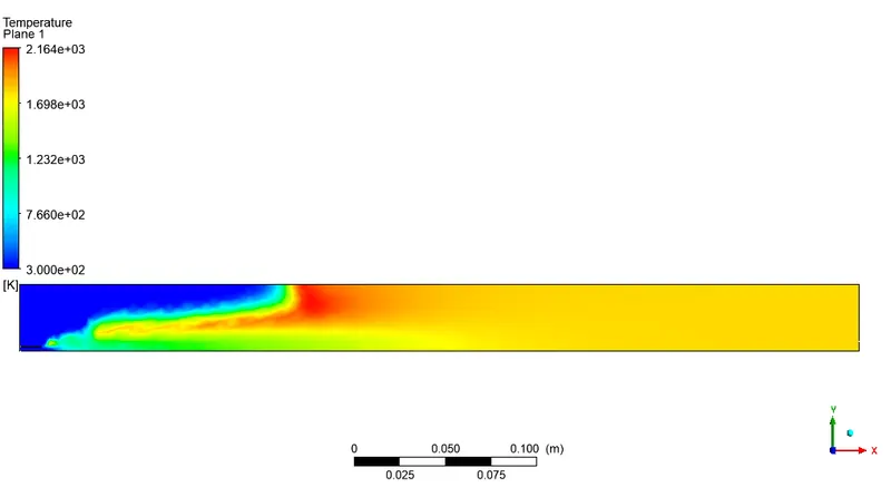
Temperature plot for 0% water addition with fuel:-
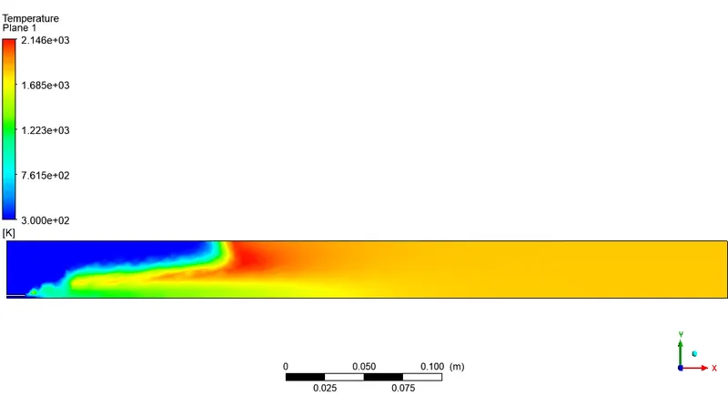
Temperature plot for 10% water addition with fuel:-
Temperature plot for 20% water addition with fuel:-
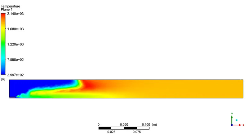
Temperature plot for 30% water addition with fuel:-
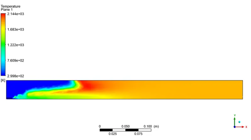
Chart plots for CH4 mass fraction at a different section of Combustor in case of adding 0%, 10%, 20%, and 30% water accordingly-
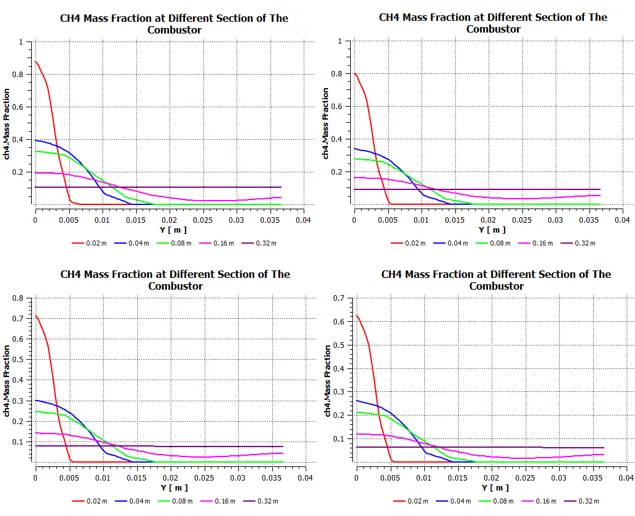
Chart plots for CO2 mass fraction at a different section of Combustor in case of adding 0%, 10%, 20%, and 30% water accordingly-
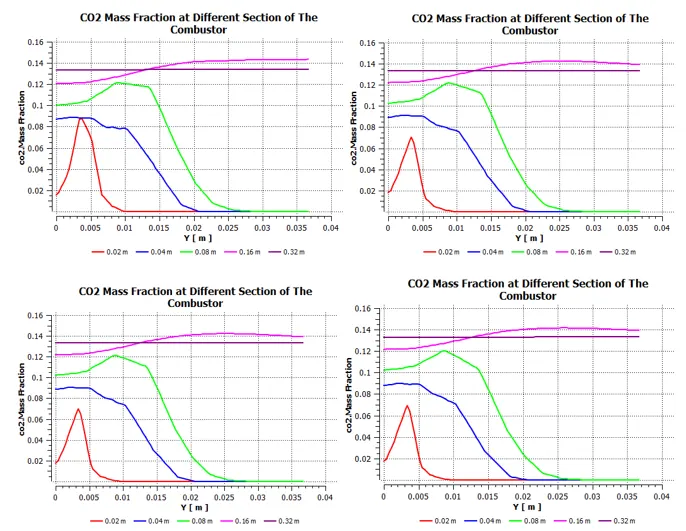
Chart plots for H2O mass fraction at a different section of Combustor in case of adding 0%, 10%, 20%, and 30% water accordingly-
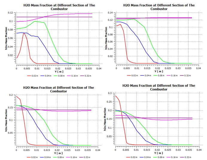
Chart plots for N2 mass fraction at a different section of Combustor in case of adding 0%, 10%, 20%, and 30% water accordingly-
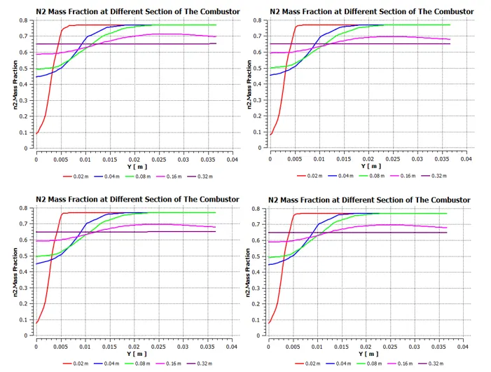
Chart plots for O2 mass fraction at a different section of Combustor in case of adding 0%, 10%, 20%, and 30% water accordingly-
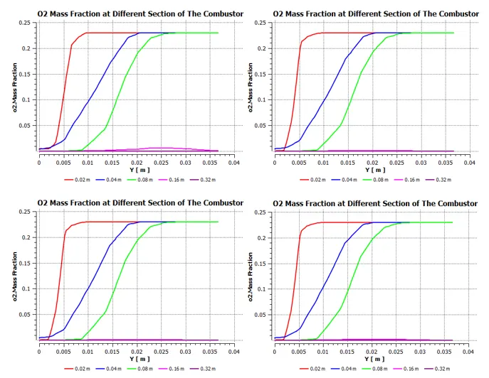
Chart plots for mass fraction of NOx emission at a different section of Combustor in case of adding 0%, 10%, 20%, and 30% water accordingly-
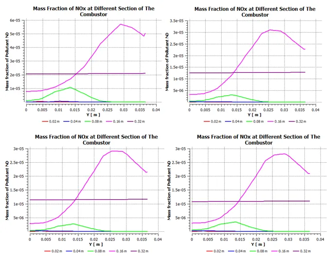
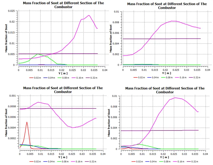
Chart plots for mass fraction of Soot at a different section of Combustor in case of adding 0%, 10%, 20%, and 30% water accordingly-
CONCLUSION:-
- Temperature plots indicate that with the addition of water, the burners' temperature decreases very little.
- Based on the chart plot, we can see that NOx emissions and soot decrease after adding water, especially after adding 20% to 30% of water. Water reduces the temperature of the burner, and the higher the temperature, the more pollutants are produced.
- There are a number of devices designed to reduce the emission of pollutants from engines and burners, but direct water injection is one of the most simple and effective ways to reduce them.