Week 10 - Simulating Combustion of Natural Gas.

Introduction:

There are two possible types of combustion simulation:

1) Based on mixing

2)Based on phase

The first catagory, based on mixing is is of three types:

1) Non premixed combustion ( Direct injection,Late injection)

2) Premixed combustion (Carburetion)

3)Partially premixed

The second catagoru that is based on phase is of four types:

1) Fluid phase ( Volumetric reaction)

2)Wall(surface reaction)

3)Particles(surface reaction)

4)Porous region(After treatment systems)

The three equations solved are the mass conservation,momentum conservation, and the species transport equation

The species transport equation is :

`(del)/(delt)((rho*Y(i))+nabla*(rho*v*Y(i))=-(nabla*j(i))+R(i)+S(i)`

Here in the above equation:

`Y(i)`= mass fraction of the species

`R(i)+S(i)`= sources. reaction and user defined

the `(del)/(delt)`term is the time derivative term.

the second term in the LHS is the convection or bulk flow term.

`-nabla*j(i)` is the diffusion term. this dictates the motion.

CFD modelling:

Flow chart :

• Geometry preparation
• Mesh generation
• Fluent set up
• Post-processing

Geometry:

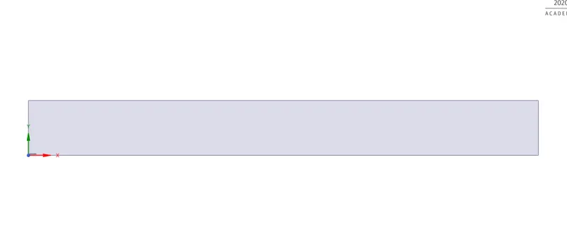
A step file of 3D combuster is opened in space claim. Due to computational restrictions, the 3D geometry is not simulated. The geometry is prepared, and a 2D geometry is prepared. The steps followed are :

1) Share : This option basically shares all the edges between the common interfaces of all the components of the geometry.

2) The 3D cylinder is split into one fourth part, This is done using the split option.

3) The projected part is copied and in a new design window , the same is pasted .

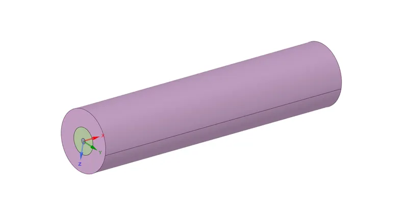
This is the 3D geometry. The final geometry that is worked upon is shown below:

• Mesh:

The modified model is transferred to the Asys mesher. Using mesh methods, triangular mesh is selected . the elemnt size provided is 1 mm.

element size	0.1 mm
elements	149833

Element quality:

minimum	0.67735
maximum	1
average	0.95014
standard deviation	4.53e-002

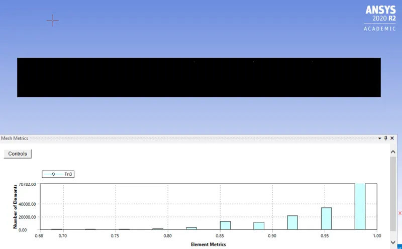
Aspect ratio:

minimum	1.001
maximum	2.274
average	1.2443
standard deviation	0.15943

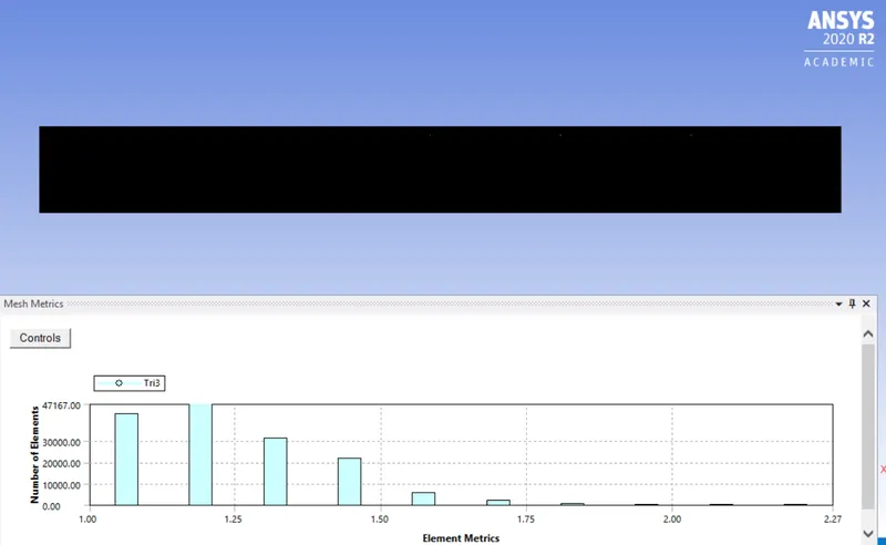
Skewness:

minimum	1.8663e-006
maximum	0.51493
average	7.31e-002
standard deviation	6.59e-002

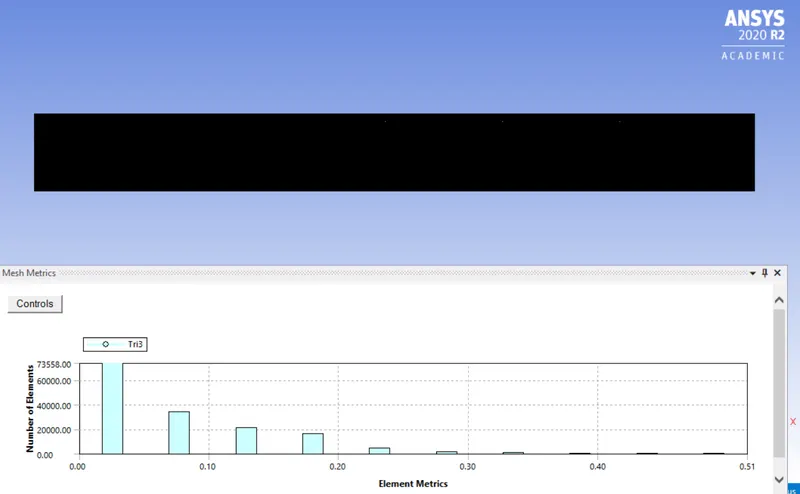
Orthogonal quality:

minimum	0.68219
maximum	1
average	0.95371
standard deviation	4.260e-002

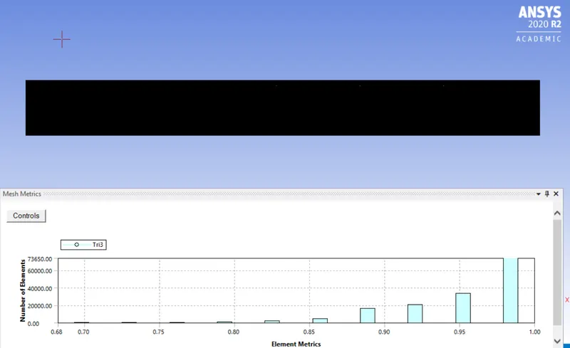
Named selection:

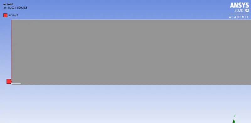
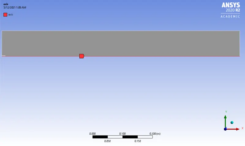
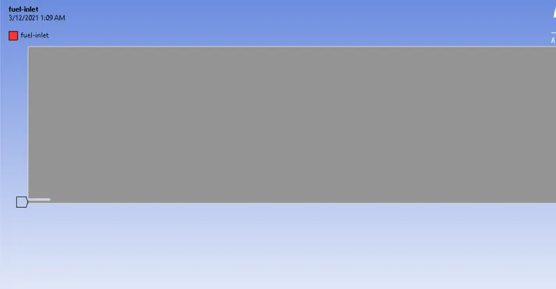
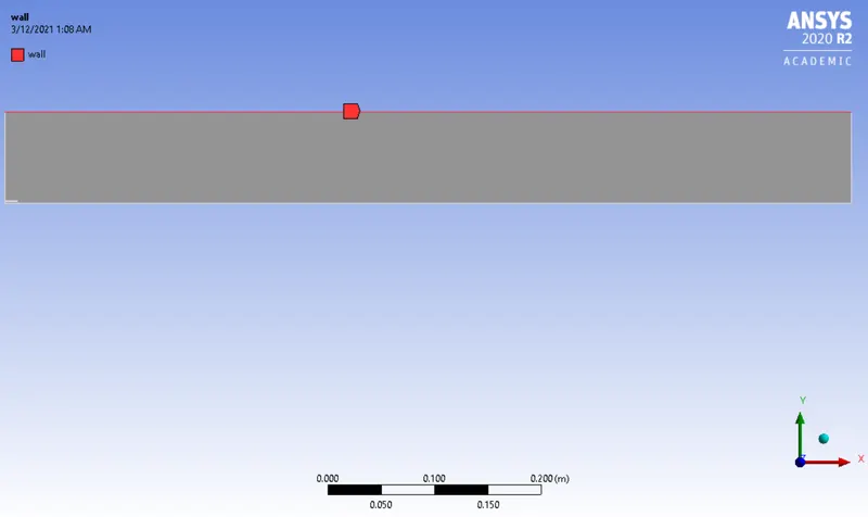
1) air inlet 2) Fuel inlet 3)Wall 4) Axis

• Fluent set up:

The meshed model is transported to fluent. Gravity is turned on. Along the Y-axis, the ccelaration due to gravity is marked -9.81m/s^2. This is an axisymmetric case . Steady state analysis is performed and pressure based solver is used.

Energy is turned on as temperature is dealt with here.

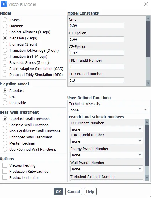
Viscous modelling:

Standard K epsilon model with standard wall functions is used.

Species modelling:

The species modelling is to set parameters related to species transport and combustion.

Species transport enables the calculation of multispecies transport either reacting or non reacting depending on type of reaction.

What Ansys Fluent does is it models mixing and transport of chemical species by solving conservation equations describing convection ,diffusion, and reaction sources for each component species.

Mixture materials - To set up the species transport and the reacting flow , a set of species and a list of rules governing their interactions are followed by mixture material selection.

• A list of constituent species reffered to as fluent materials
• A list of mixing laws to dictate how mixture properties are to be derived from property of individual species
• A set of reactions including a reaction type ( finite rate , eddy dissipation )

Eddy dissipation chemistry interaction:

Most of the fuels are fast burning and the overall rate of reaction is controlled by turbukent mixing . In non premixed flames , turbulence slowly convects or mixes fuel and oxidiser into reaction zones where they burn quickly. In premixed flames, the turbulence slowly convects cold -reactors and hot products into reaction zones where reaction occurs rapidly. such cases , combustion is said to be mixing limited to species.

The chemical reaction rate is dependent on `k/epsilon`. combustion proceeds whenever `k/epsilon`is greater than 0 and an ignition source is not required in that case for initiating combustion.

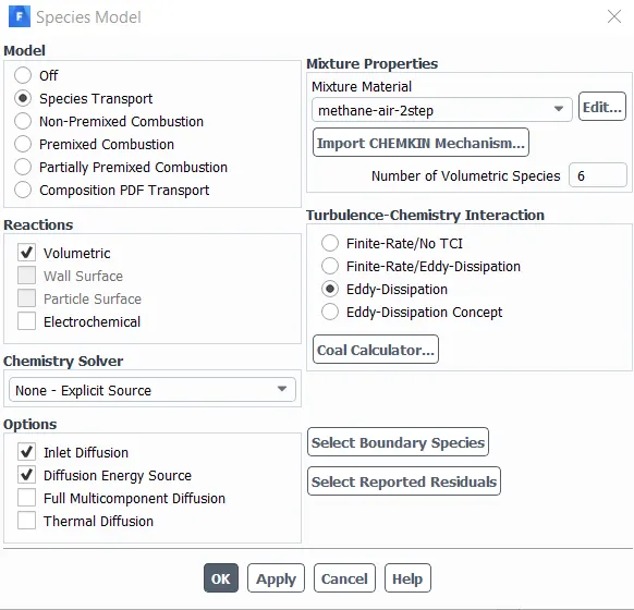
Species transport is turned on. The reaction is volumetric. Explicit source chemistry solver is opted for. Inlet diffusion and diffusion energy source is turned on. The turbulence rate chemistry interaction is eddy dissipation. As material , methane air 2 step is chosen as it allows addition of water .

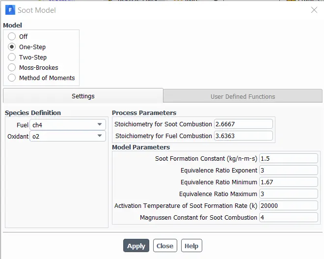
Soot model is turned on:

One step model is chosen , with species definition as methane ( CH4 )as fuel and Oxygen ( o2) as oxidant

NOx modelling:

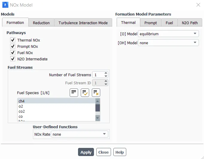
All the four pathways, Thermal NOx, Prompt NOx,FuelNOx and N2O intermediate is turned on. The primary fuel species is methane (CH4).

Bounadry Conditions:

There are two inlets , Fuel inlet and Air inlet ;

For Air inlet :

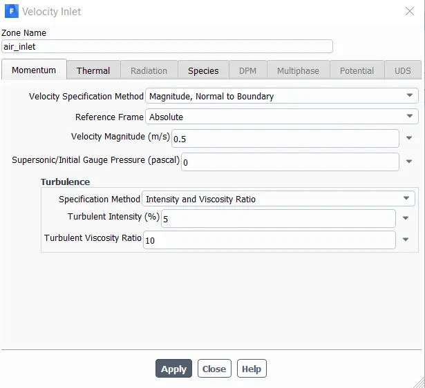
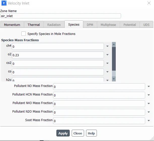
The momentum condition is, velocity of 0.5 m/s, perpendicular to the boundary , The thermal conditions are 300K and the species boundary conditions involve every species to be 0, except, oxygen(O2) which is set to 0.23 (mass fraction)

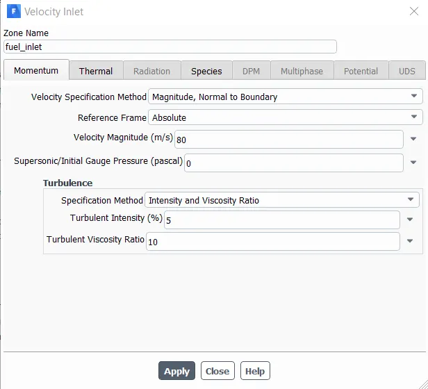
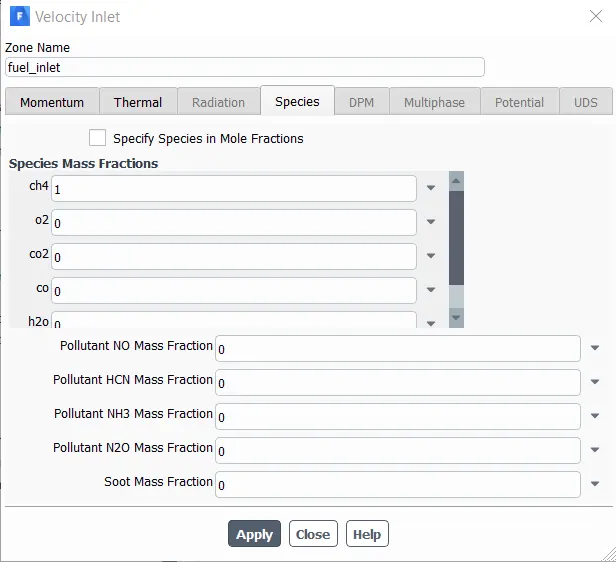
For fuel inlet :

The velocity is 80m/s , perpendicular to the boundary , the thermal condition is 300K ,

the species boundary condition is every species is set to 0 , except methane (CH4) that is the fuel species primary.

In second part of the project, water is added upto 30% .

Three xases are studied ; with 5% water, for this condition CH4 is 0.95 and H2O is 0.05 ,

With 10% water ; CH4=0.90, H2o =0.10

With 30% water ; CH4 = 0.70, H2O = 0.30

The outlet is essebntially a pressure outlet

Hybrid initialization is followed.

Contours are created for temperature ,soot and NOx formation.

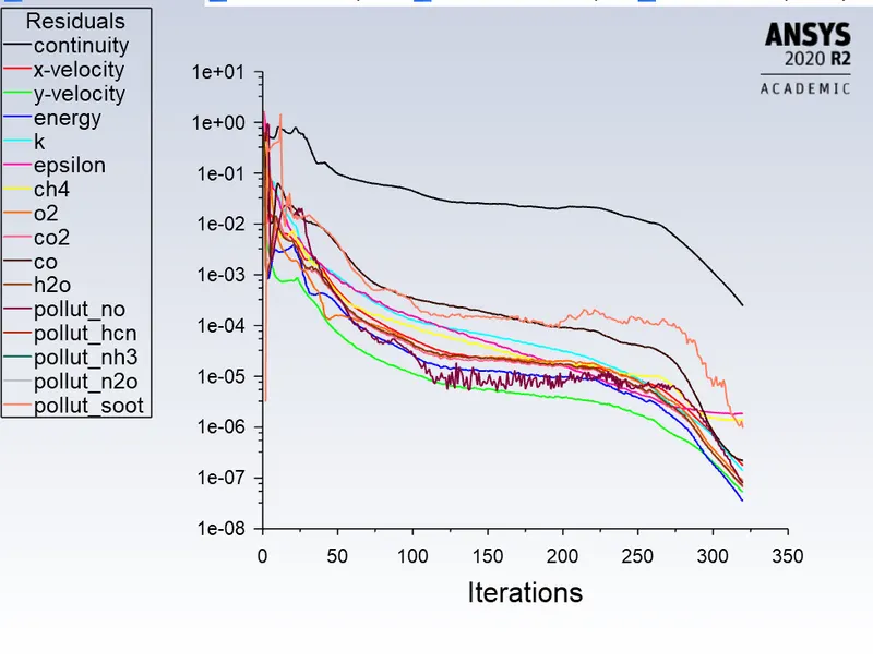
Scaled residuals :

1) without addition of water 2)with addition of water 10% 3) with addition of water 20% 4) with addition of water 30%

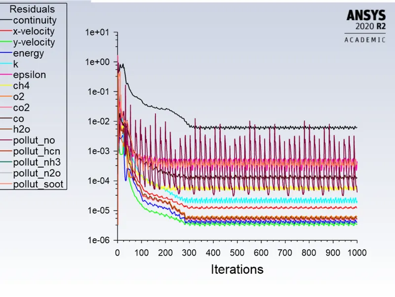
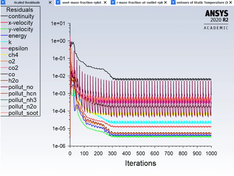
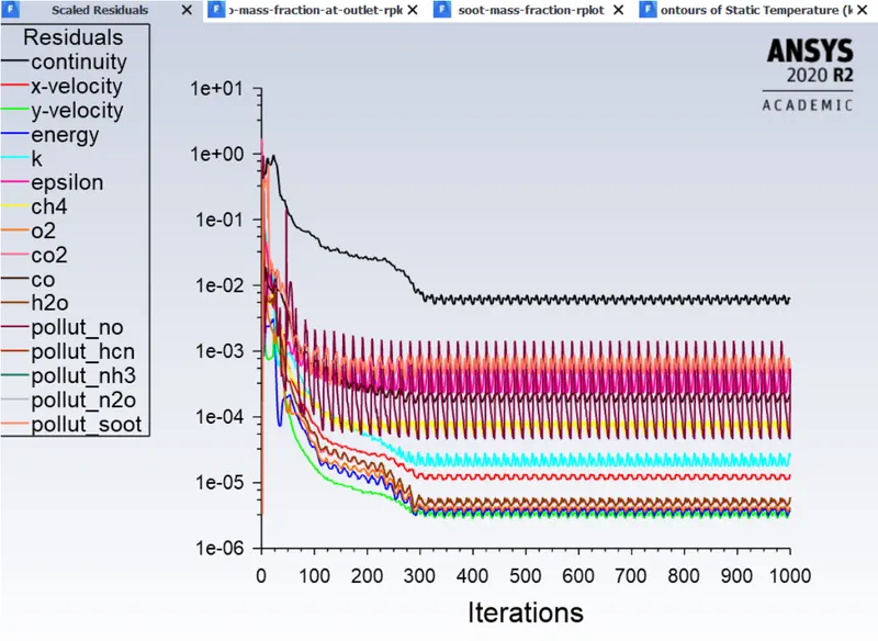
1000 iterations are set.

• Results and post processing:

The post-processing is done using the ANSYS post.

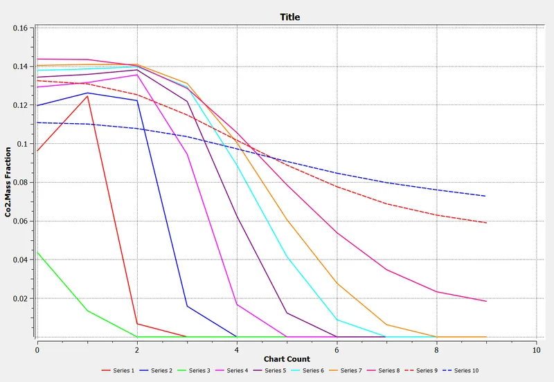
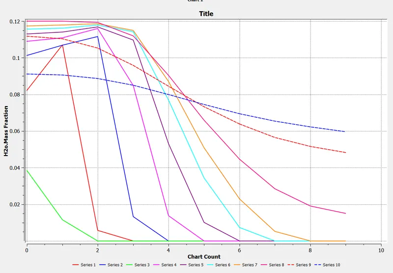
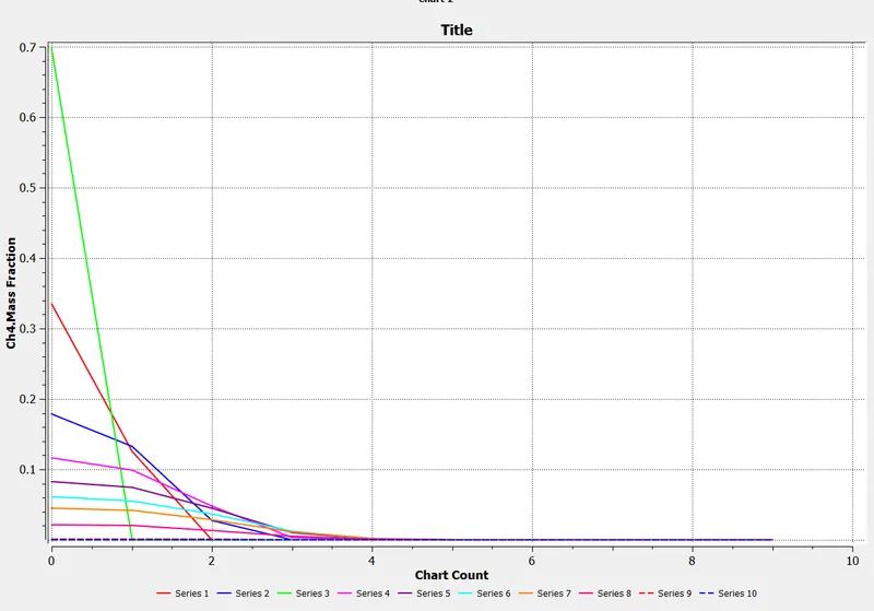
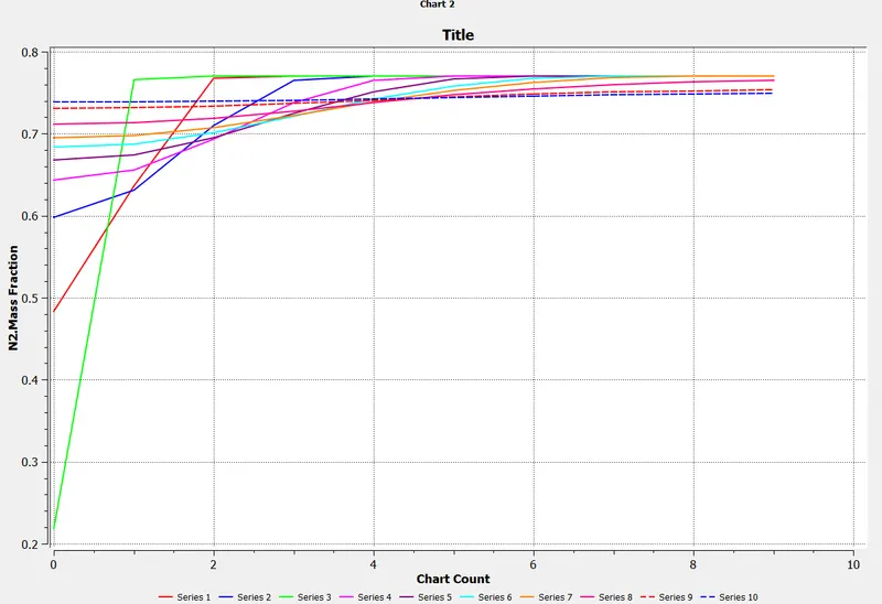
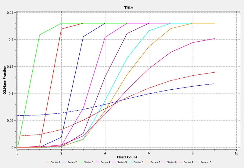
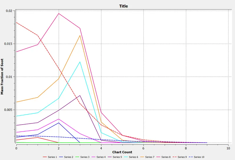
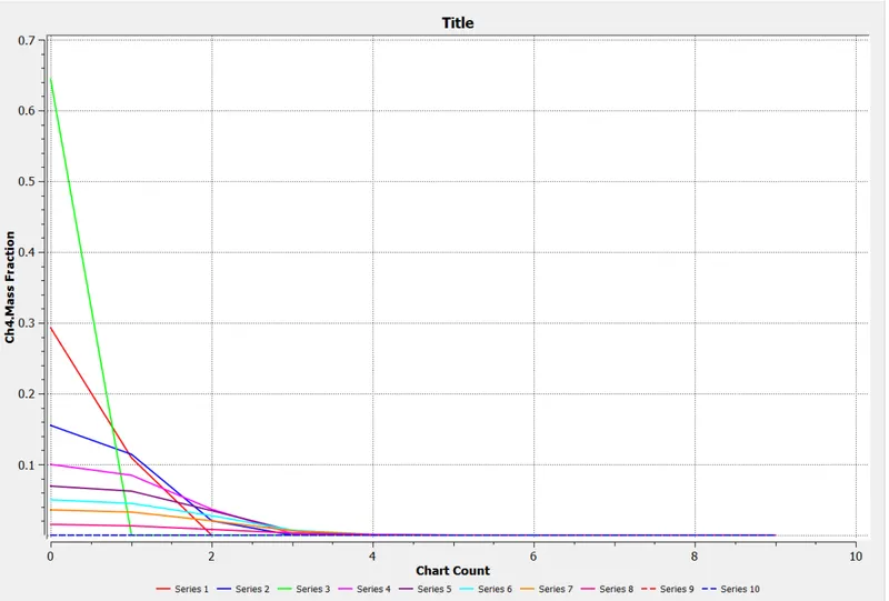
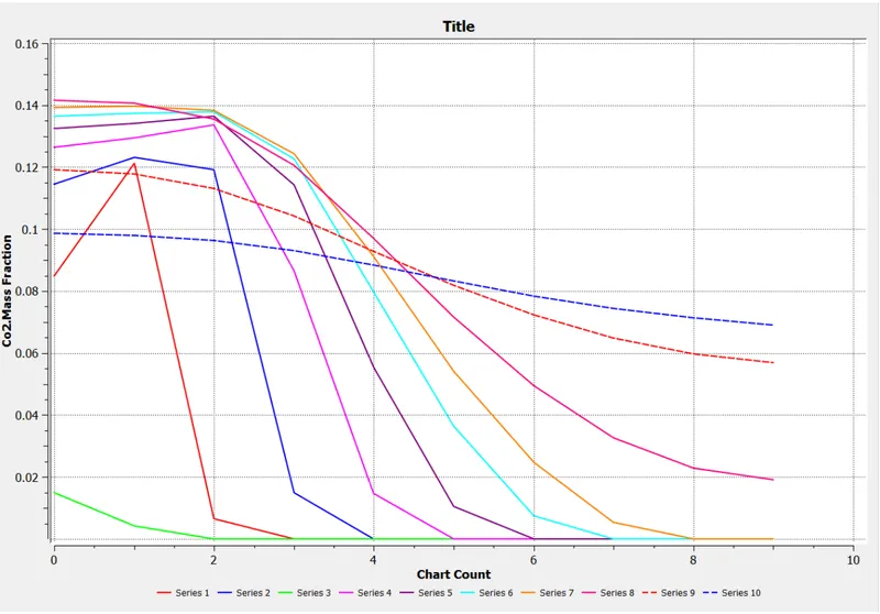
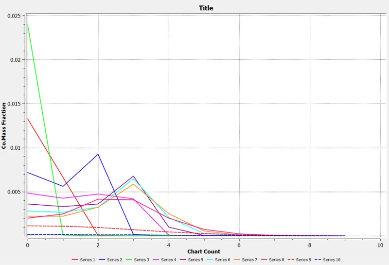
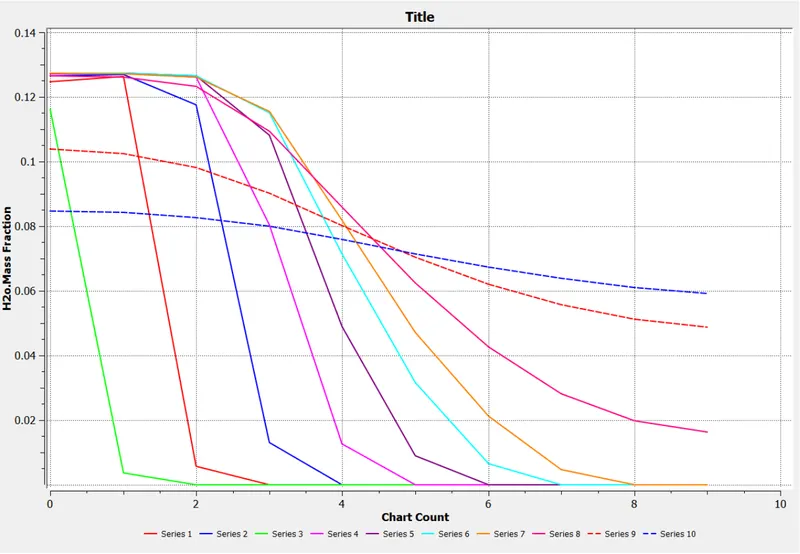
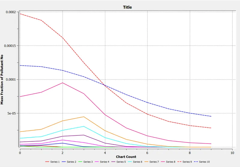
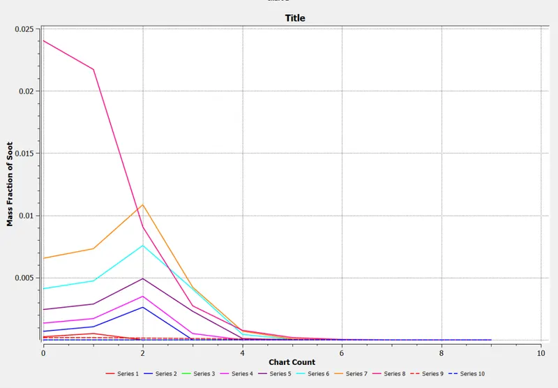
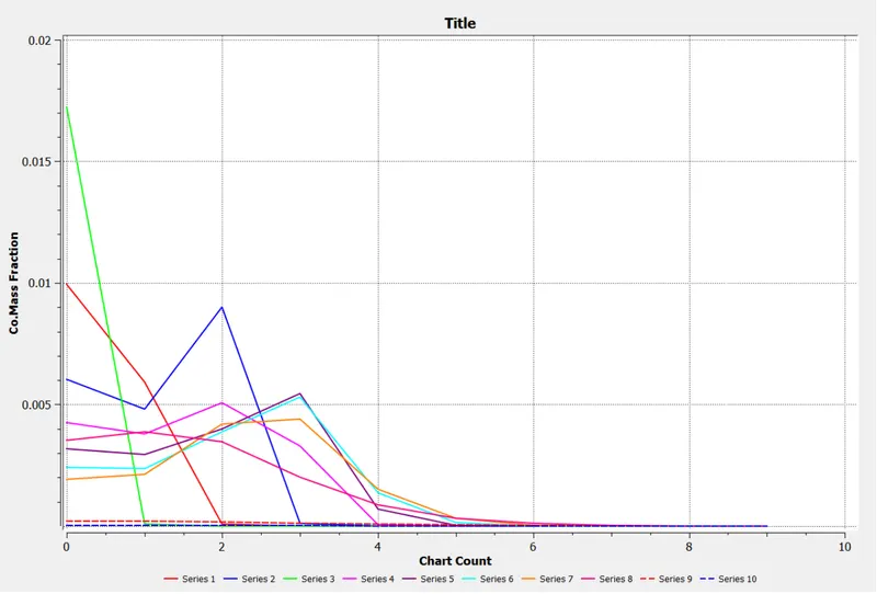
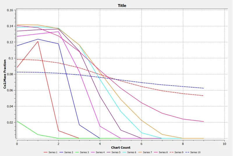
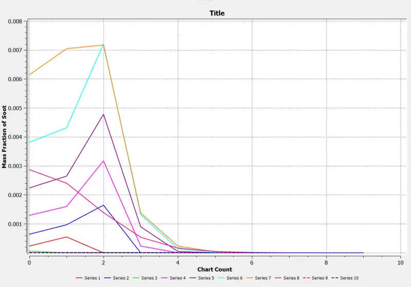
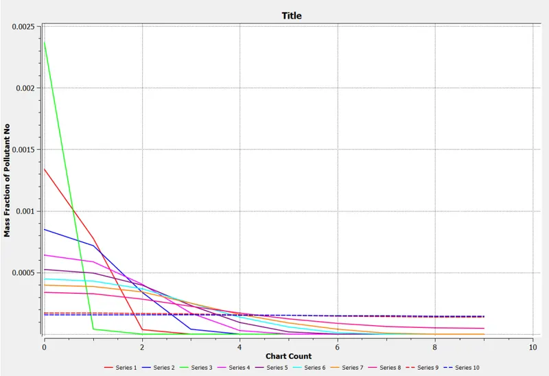
Various line probes are created inside the geometry to study or plot the mass fraction of different species. The definitions of different line probes are :

Line (1)	Two point method	(0.05,0)	(0.05,0.0852)
Line(2)	Two point method	(0.1,0)	(0.1,0.0852)
Line (3)	Two point method	(0.15,0)	(0.15,0.0852)
Line (4)	Two point method	(0.20,0)	(0.20,0.0852)
Line (5)	Two point method	(0.25,0)	(0.25,0.0852)
Line (6)	Two point method	(0.3,0)	(0.3,0.0852)
Line (7)	Two point method	(0.35,0)	(0.35,0.0852)
Line (8)	Two point method	(0.45,0)	(0.45,0.0852)
Line (9)	Two point method	(0.6,0)	(0.6,0.0852)
Line (10)	Two point method	(0.7,0)	(0.7,0.0852)

The line probes visualized like this:

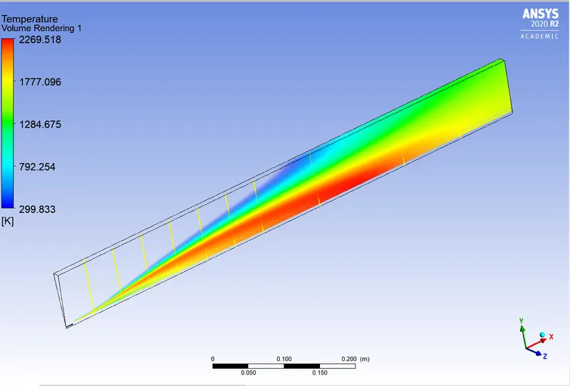
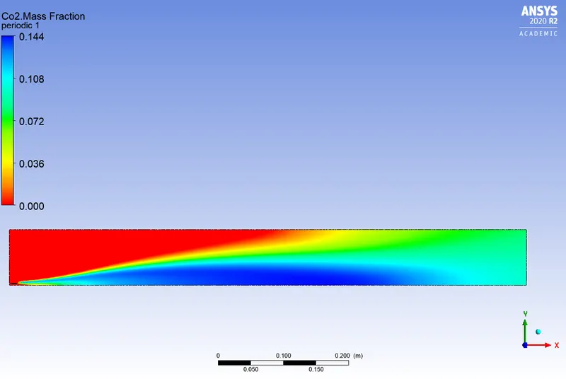
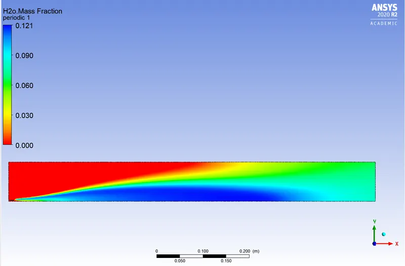
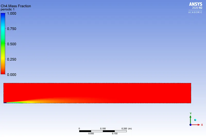
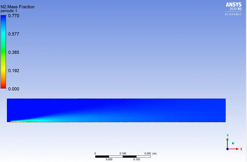
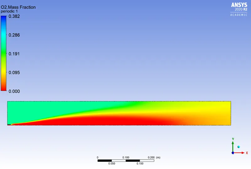
Contours are created in addition to plots of mass fraction of species . The poluutants , soot amd NO are also plotted.

1) without addition of water:

• CO2:

• H2O:

• CH4:

• N2 :

• O2:

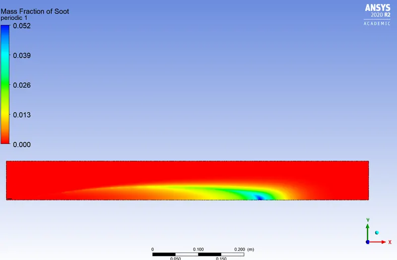
• Soot emission:

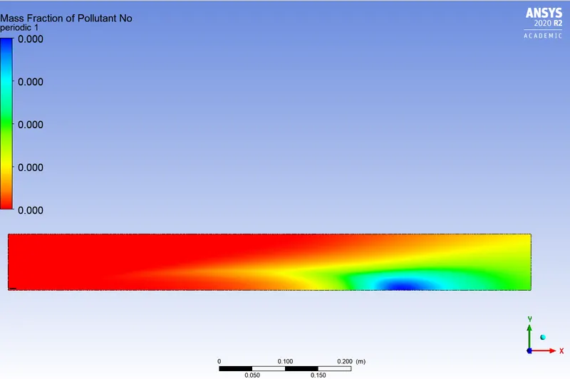
• NO emission:

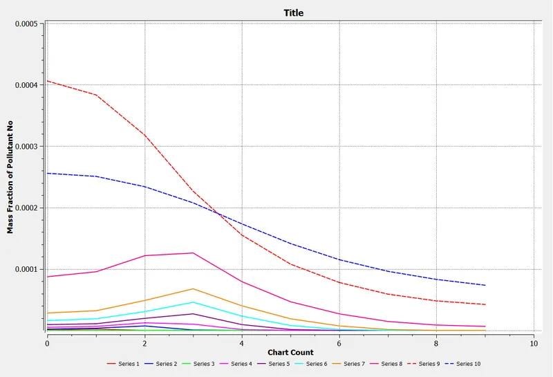
2) Water added 10% :

• O2:

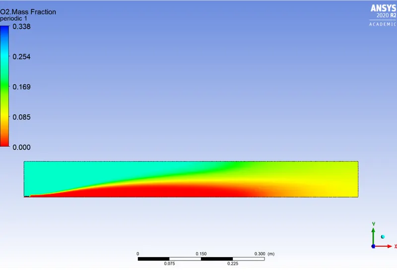
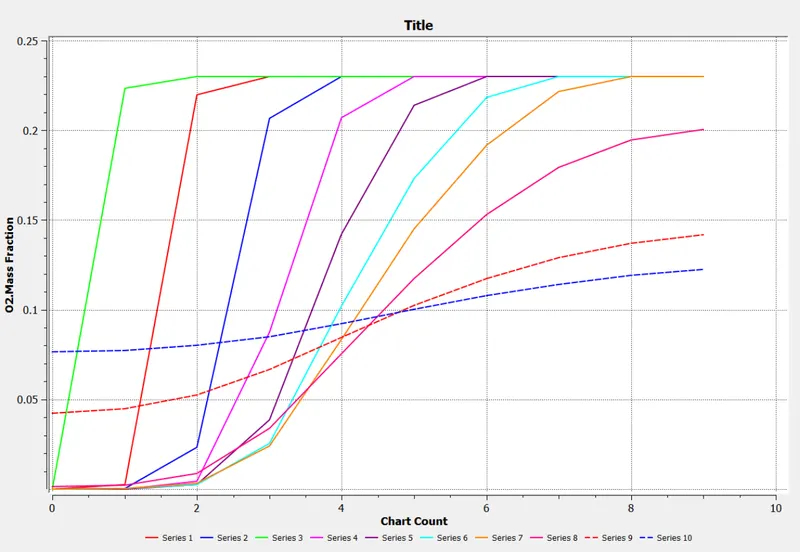
• CH4:

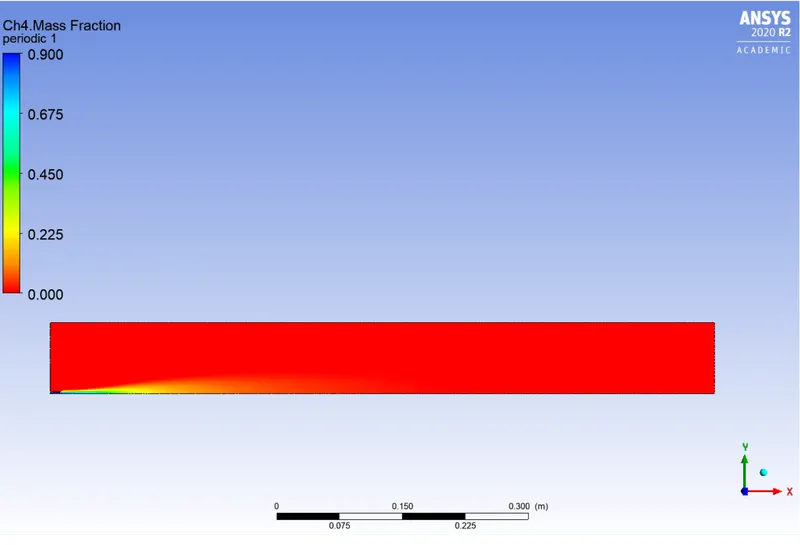
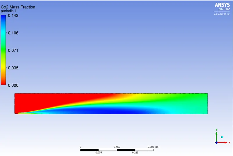
• CO2:

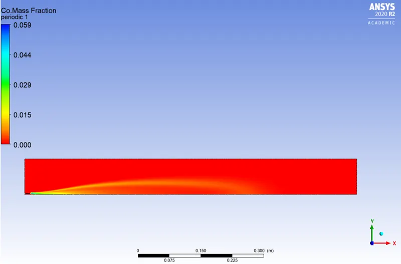
• CO:

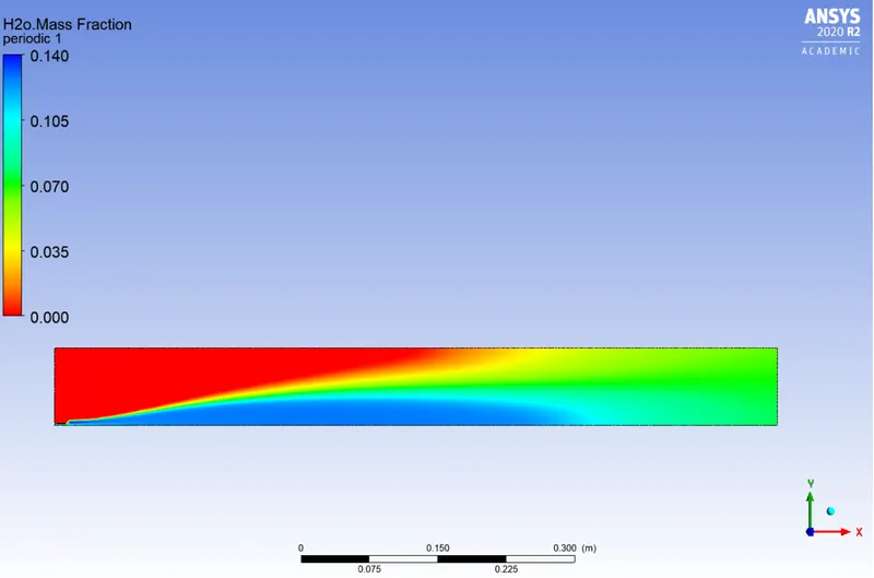
• H2O:

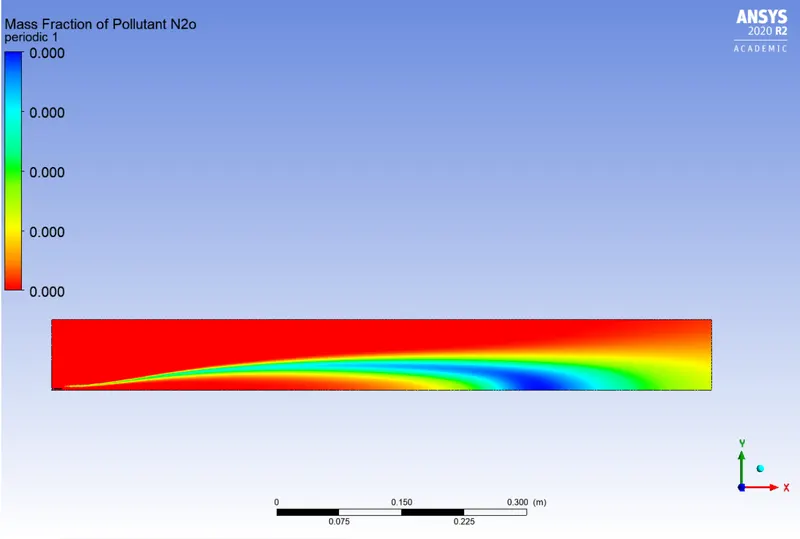
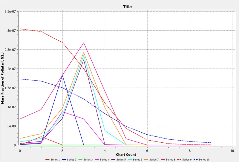
• N2O pollutant:

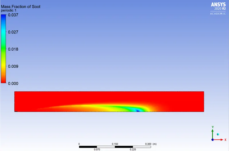
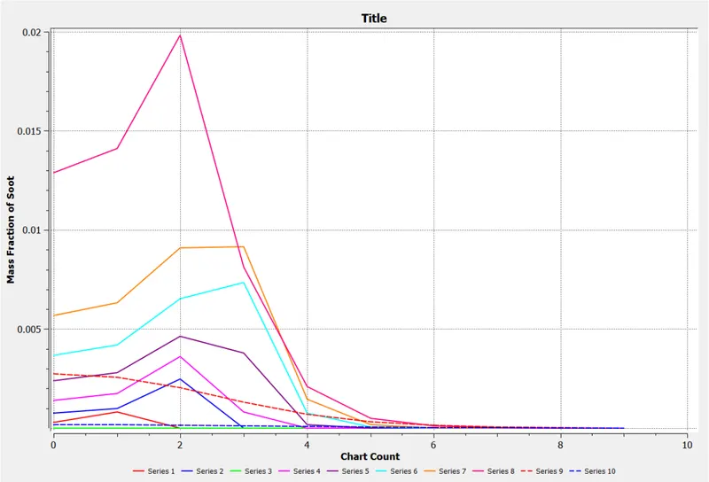
• Pollutant soot:

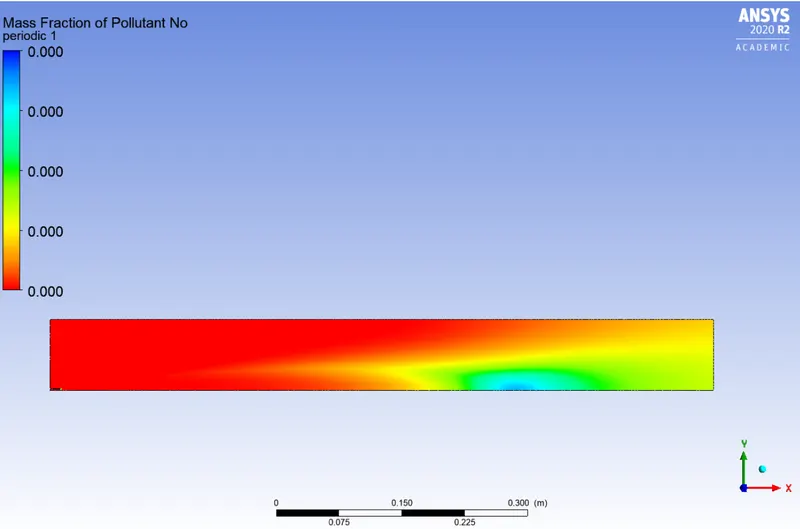
• Pollutant NO:

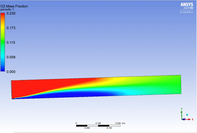
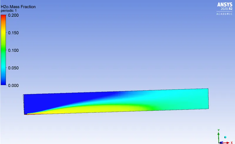
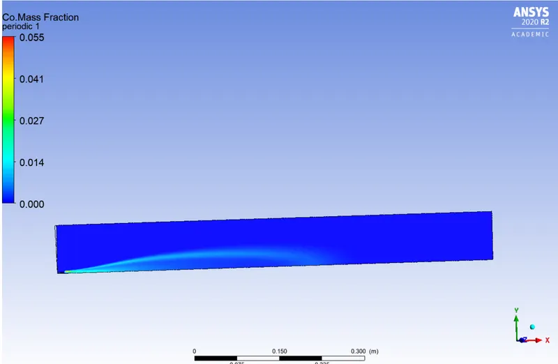
3) Water added 20%:

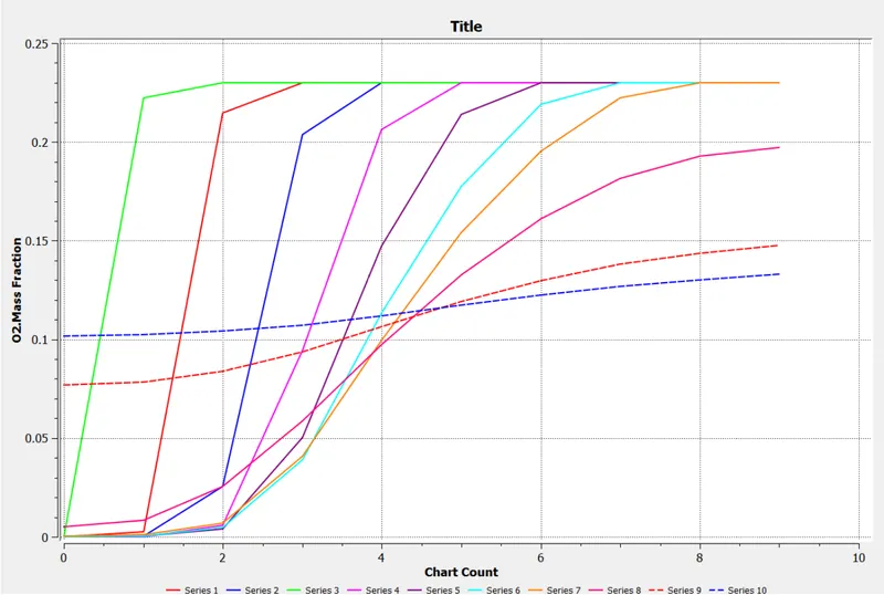
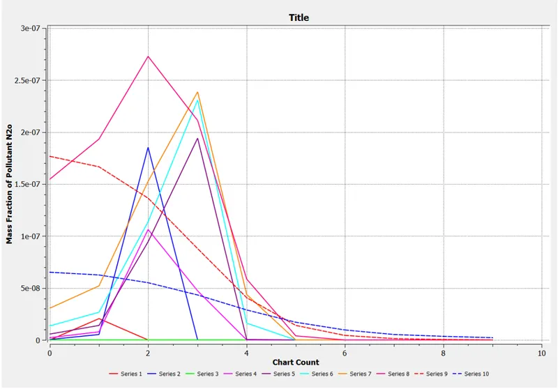
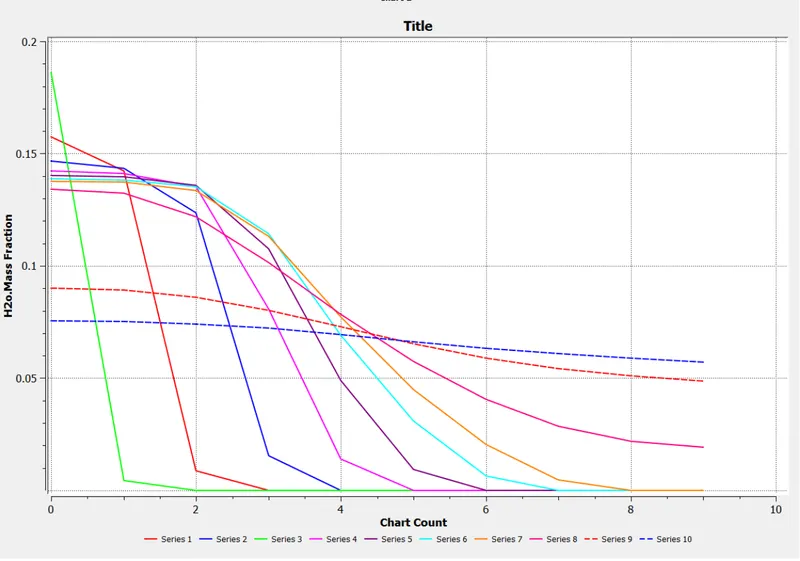
Contours of O2,H20,CO,CH4,N2,soot emission and NOx emissions are :

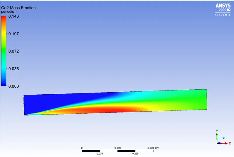
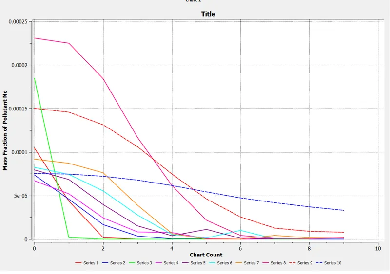
Pollutant soot and pollutant NO contours:

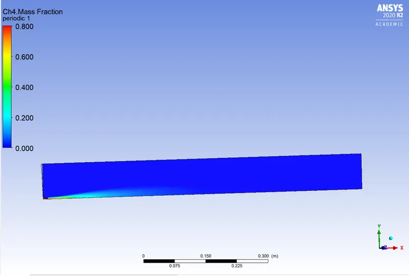
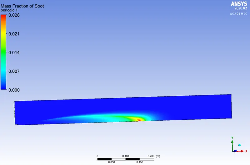
Mass fraction charts of different species :

4) Water added is 30%:

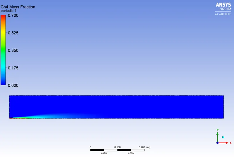
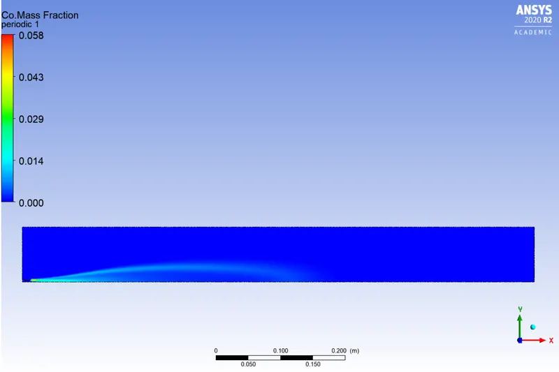
Contours of different species:

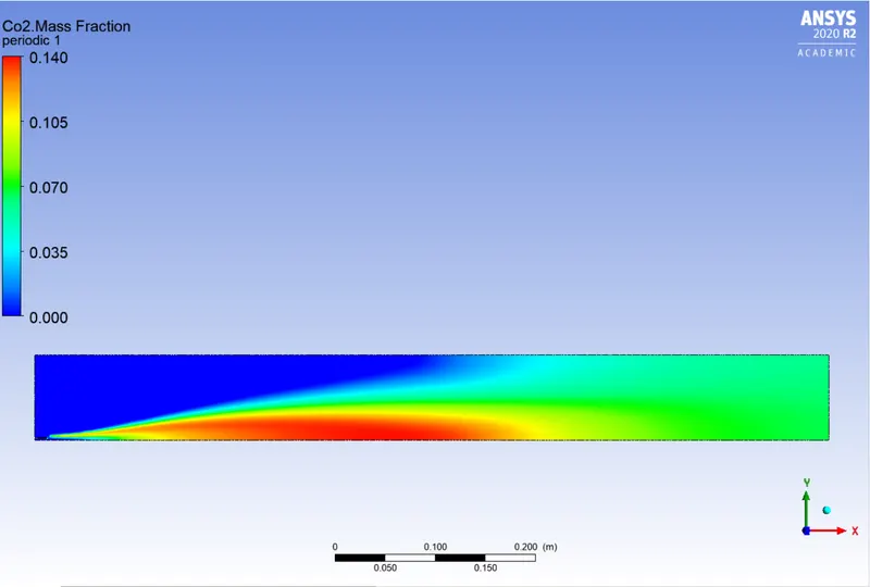
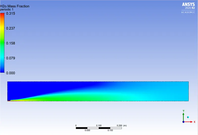
Soot and NO contours:

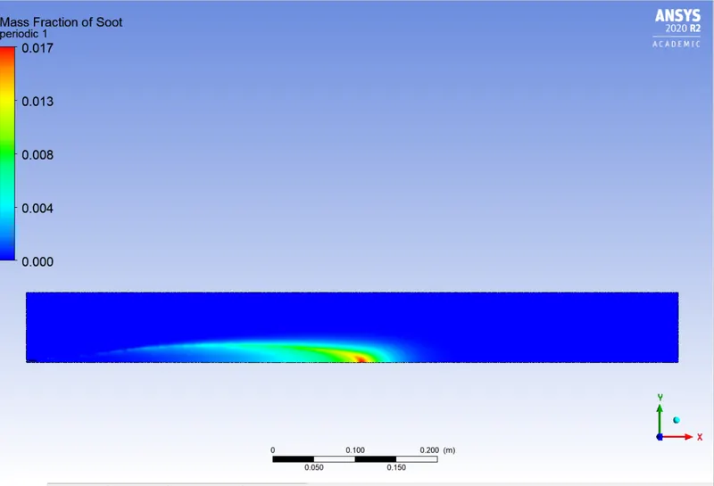
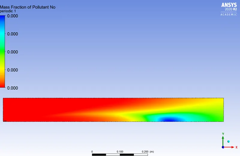
Charts of mass fraction of different species :

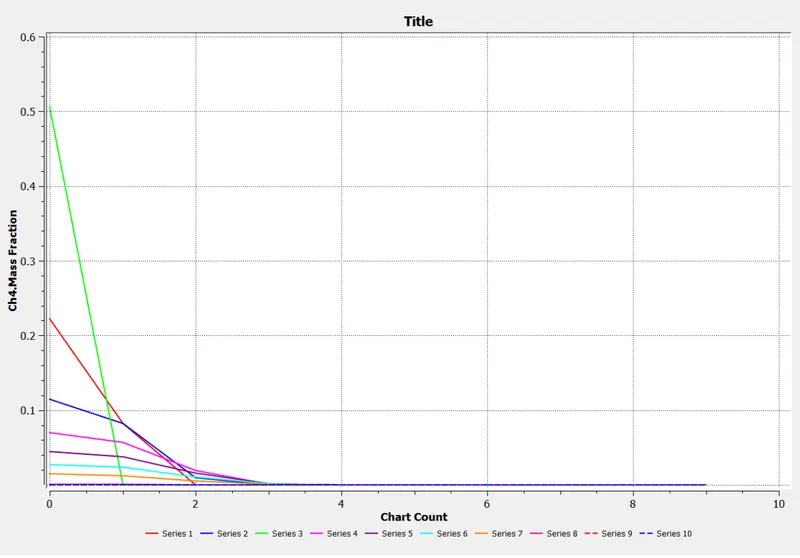
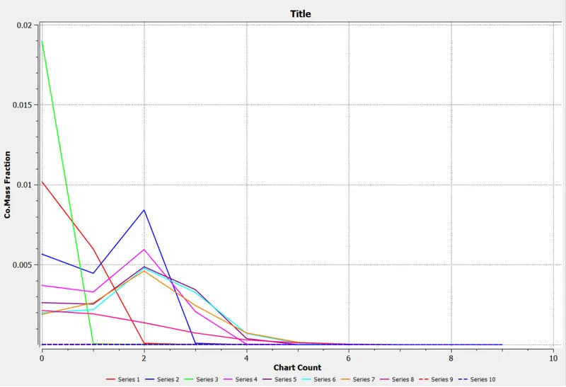
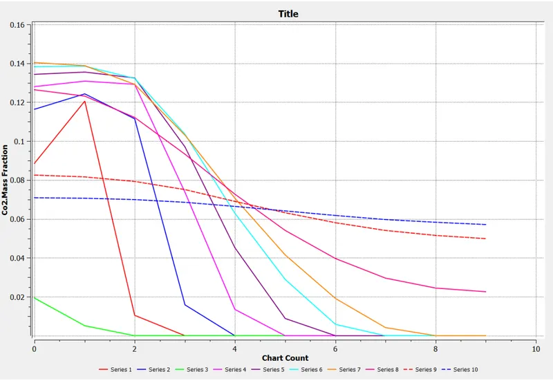
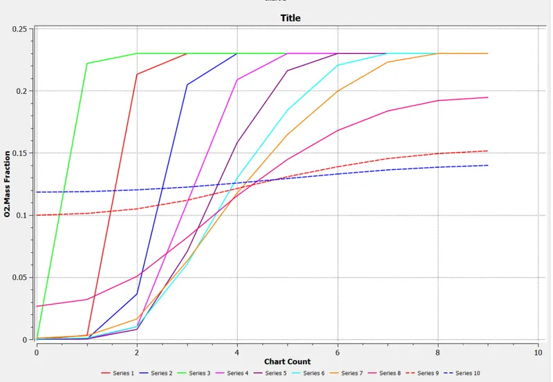
Soot and NO mass fraction chart:

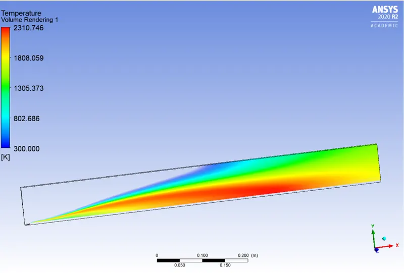
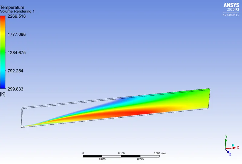
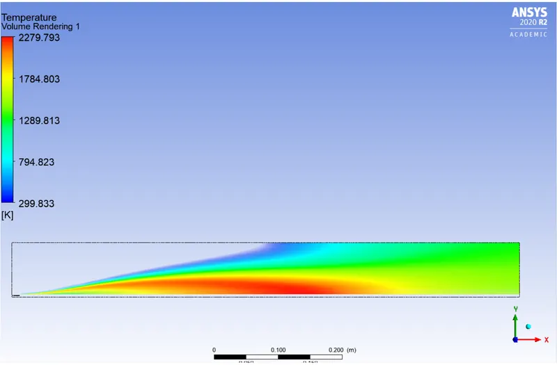
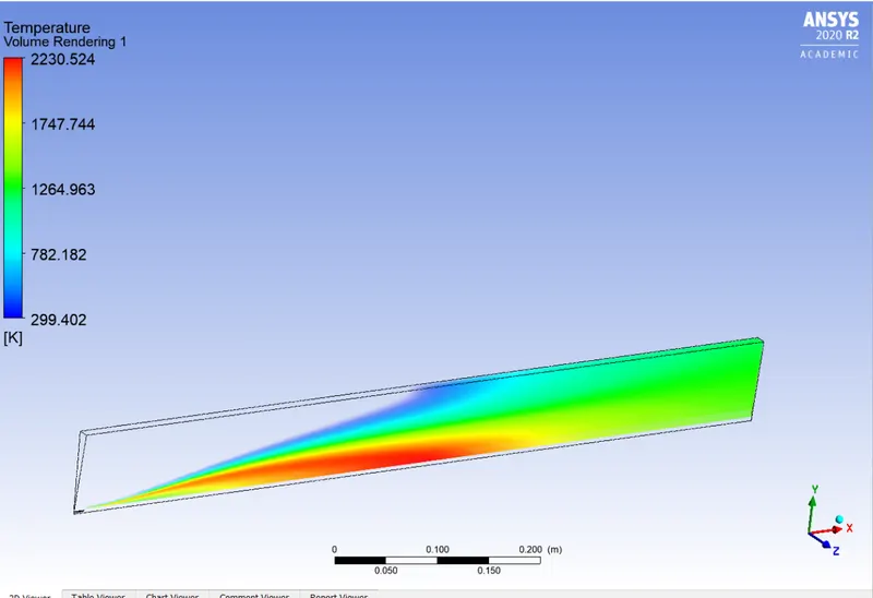
Volume rendering:

1) without water addition 2) with 10% water addition 3) with 20% water addition 4) With 30% water addition

Tabulation:

Percentage of Water	Mass fraction of Soot	Mass fraction of NO
0	4.3104e-05	4.3104e-05
10	8.0694e-06	7.2934e-05
20	5.9108e-07	7.1117e-05
30	6.7910e-08	2.1096e-05

Percentage of water added	Maximum temperature reached
0	2310.746(K)
10	2269.518(K)
20	2279.793(K)
30	2230.524(K)

Plot of soot formation and NO formation with the addition of water :

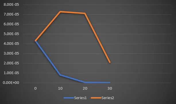
The blue curve is the soot formation curve. The orange curve is the NO formation curve. The water percentage is plotted along the X -axis , Along the Y-axis are plotted soot formation at the outlet and NO formation at the outlet.

• Conclusion:

The simulation provides a complete temperature distribution along the geometry. Contours of various species can be studied.

By adding water , the pollutant soot and NOx formation at the outlet is reduced. The plots of the same is also looked into