Week 6 - Data analysis

AIM:

File parsing

THEORY AND EXPLANATION :

File parsingis very important to find specific information from the data set. It involves opening the file , reading it and extract various data from it .

• COMPATIBILTY CHECK :

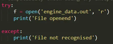
to see whether the file we are working with is compatible or ot, we use the try and except command . if the file is compatible , the file is openend , else the output shows , ' File not compatible. Please provide a valid converge file . The basic syntax is , open is the command , then within the parenthesis , we provide the name of the file first , then 'r' stands for reading the file . The file must be saved exactly in the same folder where the program is stored.

• DATA VISUALIZER:

We want to visualise the data in the file so that we can perform various functions .

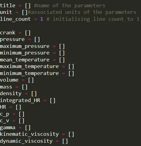
• Basic initialisations are done first. line_count is set to be 1 , empty arrays are assigned to all the parameters that are present in the file . The aim is to provide the values to all the parameters in the form of an array .

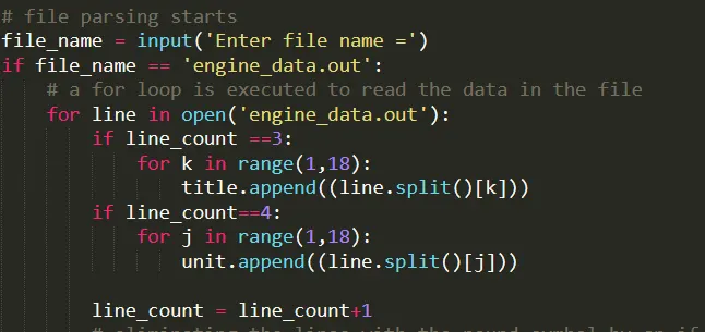
• For the file parsing , we use the for loop . First we need to enter the file name , if the file name matches the name of the file , we use the for loop to read tha data inside the file . The basic study of the data set , we tend to extract the title and the units from the third and the fourth row. also by using the if conditional statement and 'not in' we separate the lines in the file containing the '#; symbol.

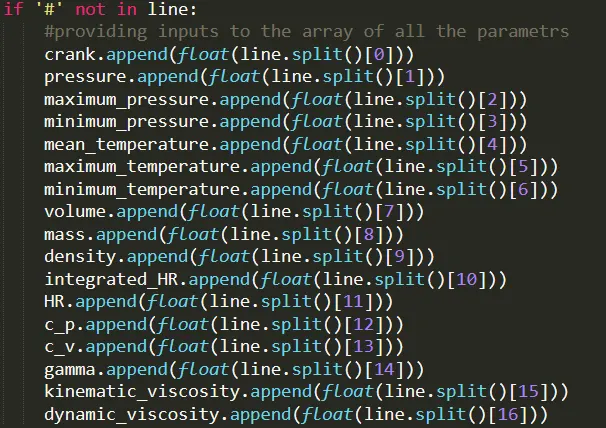
• line.split() command is used to split between the columns . to visualise the data set in the form of an array , we use the append command. all the parameters are appended with the value of them in the respective columns with the proper indexing. In python the first index starts with 0.

• An array of the properties is created using the numpy module and is assigned a variable prop. the properties are printed according to the indices.

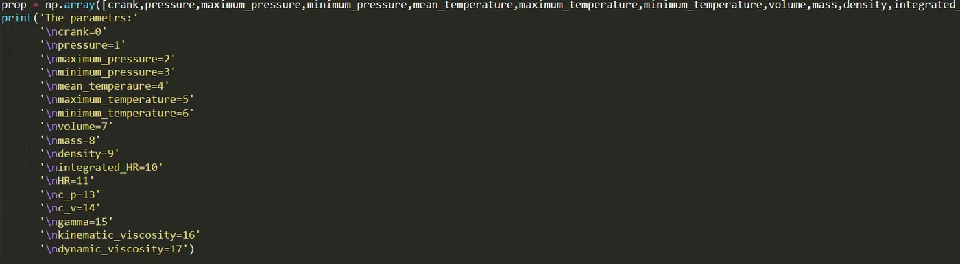
• Using the matplotlib.pyplot module the plotting is performed. we are expected to enter an index for the property we want to see in the x axis and similarly for the property we want to see on the y axis. Using the savefig() command the plots are saved. The plot is showed on the screen using the plt.show() command

• ENGINE PERFORMANCE CALCULATION :

For Volume in x axis and pressure in y axis , we first need to create the plot. Then Work done by the engine needs to found out. work done is basically the area under the p-v diagram. RPM of the engine is given in the problem as 1500 . Power developed by the engine is calculated from the formula P = 2*pi*N*T/(60*1000) , Here N is the rpm provided . Engine fuel consumption i provided in micro grams per second. the specific fuel consumption is found out.

simps command is used to find out the area under the p-v diagram. The simps command is from the scipy.integrate . it basically uses the simpsons rule to compute the integral.

The graph is plotted with volume in the x axis and pressure in the y axis .

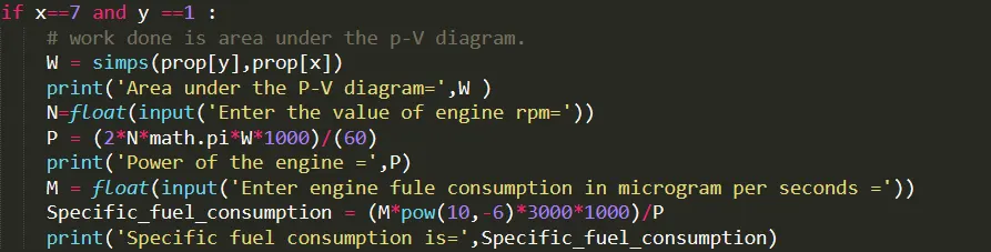
The python code for the complete project is pasted below:

import matplotlib.pyplot as plt
import numpy as np
import math
from scipy.integrate import simps
# compatibilty check using try except command
try:
    f = open('engine_data.out', 'r')
    print('File openend')

except:
    print('File not recognised')
    
# basic initialisations
# assigning empty arrays to all the parameters

title = [] #name of the parameters
unit = []#associated units of the parameters
line_count = 1 # initialising line count to 1

crank = []
pressure = []
maximum_pressure = []
minimum_pressure = []
mean_temperature = []
maximum_temperature = []
minimum_temperature = []
volume = []
mass = []
density = []
integrated_HR = []
HR = []
c_p = []
c_v = []
gamma = []
kinematic_viscosity = []
dynamic_viscosity = []

# file parsing starts
file_name = input('Enter file name =')
if file_name == 'engine_data.out':
    # a for loop is executed to read the data in the file 
    for line in open('engine_data.out'):
        if line_count ==3:
            for k in range(1,18):
                title.append((line.split()[k]))
        if line_count==4:
            for j in range(1,18):
                unit.append((line.split()[j]))

        line_count = line_count+1 
        # eliminating the lines with the pound symbol by an if statement and using ' not in' 
        if '#' not in line:
            #providing inputs to the array of all the parametrs 
            crank.append(float(line.split()[0]))
            pressure.append(float(line.split()[1]))
            maximum_pressure.append(float(line.split()[2]))
            minimum_pressure.append(float(line.split()[3]))
            mean_temperature.append(float(line.split()[4]))
            maximum_temperature.append(float(line.split()[5]))
            minimum_temperature.append(float(line.split()[6]))
            volume.append(float(line.split()[7]))
            mass.append(float(line.split()[8]))
            density.append(float(line.split()[9]))
            integrated_HR.append(float(line.split()[10]))
            HR.append(float(line.split()[11]))
            c_p.append(float(line.split()[12]))
            c_v.append(float(line.split()[13]))
            gamma.append(float(line.split()[14]))
            kinematic_viscosity.append(float(line.split()[15]))
            dynamic_viscosity.append(float(line.split()[16]))
    # an array of all the properties is created and assigned to a variable prop . The properties are printed in a tabular form . the index value showing the column numbers.
    prop = np.array([crank,pressure,maximum_pressure,minimum_pressure,mean_temperature,maximum_temperature,minimum_temperature,volume,mass,density,integrated_HR,HR,c_p,c_v,gamma,kinematic_viscosity,dynamic_viscosity])
    print('The parametrs:'
          '\ncrank=0'
          '\npressure=1'
          '\nmaximum_pressure=2'
          '\nminimum_pressure=3'
          '\nmean_temperaure=4'
          '\nmaximum_temperature=5'
          '\nminimum_temperature=6'
          '\nvolume=7'
          '\nmass=8'
          '\ndensity=9'
          '\nintegrated_HR=10'
          '\nHR=11'
          '\nc_p=13'
          '\nc_v=14'
          '\ngamma=15'
          '\nkinematic_viscosity=16'
          '\ndynamic_viscosity=17')


    #plotting the graphs between different parameters . And also any two combinations of columns can be taken.
    x = int(input('Enter the property on x-axis ='))
    y = int(input('Enter the property on y-axis= '))
    plt.plot(prop[x],prop[y])
    plt.xlabel((title[x])+(unit[x]))
    plt.ylabel((title[y])+(unit[y]))
    plt.title('Plot of '+title[x]+ 'v' +title[y])
    plt.savefig(title[x]+ 'v' +title[y]) # to save the figures separately
    plt.show()



    # engine performance calculation
    # providing condition to pick the pressure column in 
    if x==7 and y ==1 :
        # work done is area under the p-V diagram.
        W = simps(prop[y],prop[x])
        print('Area under the P-V diagram=',W )
        N=float(input('Enter the value of engine rpm='))
        P = (2*N*math.pi*W*1000)/(60)
        print('Power of the engine =',P)
        M = float(input('Enter engine fule consumption in microgram per seconds ='))
        Specific_fuel_consumption = (M*pow(10,-6)*3000*1000)/P
        print('Specific fuel consumption is=',Specific_fuel_consumption)




   

OUTPUT:

1. 

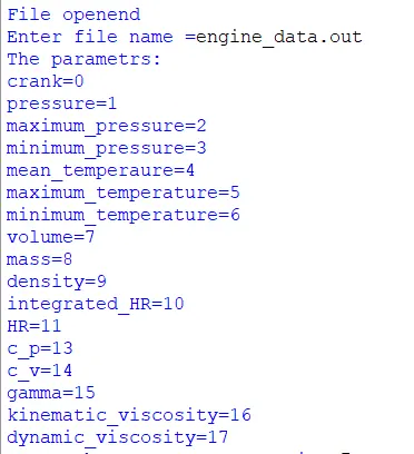
The above image shows that file opened . so the compatabilty check is done and it came out to be correct . The file name is enterred and the parameters are printed with correct indices .

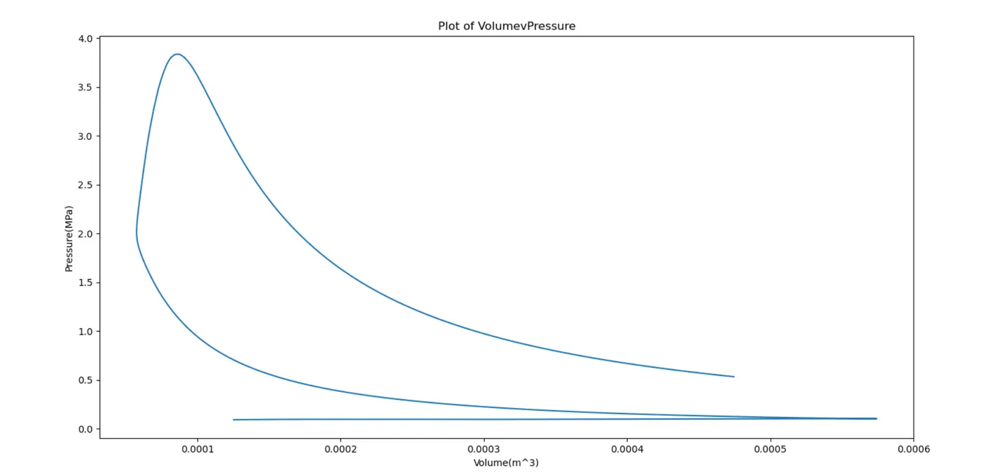
The plot is obtained between pressure in y axis and the volume in x axis. similarly by providing the indices in x and y ac=xis we can get plots between different parameters also.

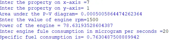
The area under the p-v diagram came out to be 0.00050058 *10^6 joules

The power of the engine as 78.63 kw

The Specific fuel consumption as 0.7630 kg/kw-h

CONCLUSION :

• data analysis provides us with a tool to compare different parameters and performance . It helps in task automation.
• Specific fuel consumption reflects the efficiency of an engine.