Week 5 - Curve fitting

AIM :

To perform curve fitting

THEORY :

Curve fitting is the way we model or represent a data spread by assigning a best fit function (curve) along the entire range. Ideally, it will capture the trend in the data and allow us to make predictions of how the data series will behave in the future.

There are two types of curve fitting :

1) Interpolation : where you discover a function that is an exact fit to the data points. Since this assumes no measurement error, it has limited applicability to real life scenarios.

2) Smoothing : It is when we find a function that is an approximate fit to the data points, but we give room for error and we allow our actual points to be near, but not necessarily on the line; given the error is minimized overall .

What does popt and pcov mean?

popt stores the coefficients that are calculated by the curve_fit function. It is a output .

pcov stores the estimated co variance in the popt values . This is also a output. This is a 2D array

What does *in*popt means?

It means that the coefficients values of a,b,c,d,e,f are stored in array form in popt. * this is used to referto these values .

What needs to be done to make the fit perfect ?

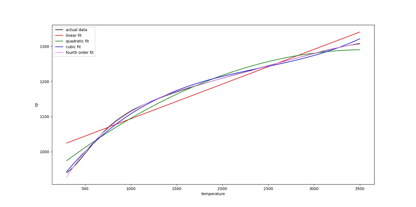
From the outputs it is seen that the higher the order of polynomial , better and more accurate is the fit.

The Good ness of the curve fit is estimated by four methods :

1) Sum of squares due to error

2) R-square

3) adjusted R -square

4) Root mean squared error

EXPLANATION OF CODE AND VARIOUS COMMANDS :

To perform a curve fit , the numpy module , matplotlib module and the scipy module needs to be imported. Moreover if some statistics operation is to be performed , the statistics module is also to be imported.

• import matplotlib.pyplot as plt
• import numpy as np
• from scipy.optimize import curve_fit
• from statistics import mean

A function is now defined that will be called at various stages of the code . the function can be a linear one if we intend to fit a linear equation, a qudratic one or a cubic one and it is returned . The function model takes in the independent variable in the first place , then the coefficients or argu,ents accordingly .

• def linfunction (t,a,b):
• return a*t+b

A function read_file() is called. The read_file() function reads the data file . Here the data file contains temperature and specific heat values. The temperature and specific heat is assigned empty arrays so theat the values are generated afterwards.

• def read_file():
• temperature = []
• cp = []

We have to open a file called data . The data file needs to be stored in the same folder containing the program file. The 'r' command refers to read mode. It means we are opening the data file and reading its contents .

• for line in open('data','r'):

for each line in the data file we are running a command to split the line in two parts. One part containing the temperature values and another one the cp values . Split command is used.

• values = line.split(',')

To generate the arrays for temperature and the cp values. We append those using float values. 0 for the first column, 1 for the second column.

• temperature.append(float(values[0]))
• cp.append(float(values[1])

The temperature and cp is returned

• return[temperature,cp]

The curve_fit command takes in the model function, the temperature and the cp values . the model function is the mathematical model we are using to represent our data.

• curve_fit(linfunction,temperature,cp)

We get two outputs here ; popt and pcov ,

Popt: This represents the coefficients that are calculated by the curve_fit function .

pcov: This is the estimated co-variance of the popt values.

• popt,pcov1 = curve_fit(linfunction,temperature,cp)

As we have our new coefficients values calculated , we consider the function again , then we pass the temperature array along the coefficients .

• fit_cp1 = linfunction(np.array(temperature),*popt)

We pass the entire temperature as am array so , the np.array(temperature)

instead of passing the coefficient values we are passing the popt . It takes care of the co efficients.

The results are plotted using the matplotlib.pyplot module.

Now , the following program has three parts :

1) the curve fit program is performed for linesr fit, quadratic fit , cubic equation, and fourth order equation.

2) the results are plotted

3) to evaluate the goodness of fit by R^2 method and RMSE values

import numpy as np
import matplotlib.pyplot as plt
from scipy.optimize import curve_fit
import math
from statistics import mean


def linfunction (t,a,b):
    return a*t+b 
def quadfunction(t,a,b,c):
	return a*pow(t,2)+b*t+c

def cubicfunction (t,a,b,c,d):
	return a*pow(t,3)+b*pow(t,2)+c*t+d

def fourthpowerfunction (t,a,b,c,d,e):
	return a*pow(t,4)+b*pow(t,3)+c*pow(t,2)+d*t+e




#file reading 
def read_file():
    temperature=[]
    cp=[]
    for line in open('data','r'):
        values = line.split(',')
        temperature.append(float(values[0]))
        cp.append(float(values[1]))
    return[temperature,cp]

#curve fitting of linear function
temperature,cp = read_file()
popt,pcov1 = curve_fit(linfunction,temperature,cp)
fit_cp1 = linfunction(np.array(temperature),*popt)


#curve fitting of quadratic function
temperature,cp = read_file()
popt,pcov2 = curve_fit(quadfunction,temperature,cp)
fit_cp2 = quadfunction(np.array(temperature),*popt)

#curve fitting of cubic function 
temperature,cp = read_file()
popt,pcov3 = curve_fit(cubicfunction,temperature,cp)
fit_cp3 = cubicfunction(np.array(temperature),*popt)

#curve fitting of fourth power function
temperature,cp = read_file()
popt,pcov4 = curve_fit(fourthpowerfunction,temperature,cp)
fit_cp4= fourthpowerfunction(np.array(temperature),*popt)

#plotting the curve_fit data 

plt.plot(temperature,cp,'black',linewidth=1.5,label='actual data')
plt.plot(temperature,fit_cp1,'red',linewidth=1.5,label='linear fit') #linear curve_fit
plt.plot(temperature,fit_cp2,'green',linewidth=1.5,label='quadratic fit') #quadratic curve_fit
plt.plot(temperature,fit_cp3,'blue',linewidth=1.5,label='cubic fit')#cubic curve_fit
plt.plot(temperature,fit_cp4,'violet',linewidth=1.5,label='fourth order fit') #fourth power curve_fit 
plt.legend()
plt.xlabel('temperature')
plt.ylabel('cp')
plt.show()


#finding the best fit by different methods 




def R_square (temperature,cp,fit_cp):
    for i in range (0,len(temperature)):
	    Mean = mean(cp)
	    SSR = np.sum((fit_cp[i]-Mean)**2)
	    SSE = np.sum((cp[i]-fit_cp[i])**2)
	    SST = SSE + SSR 
	    r_2= SSR/SST
    return r_2

#evaluating for differnt order fits

R11 = R_square (temperature,cp,fit_cp1)
R12 = R_square (temperature,cp,fit_cp2)
R13 = R_square (temperature,cp,fit_cp3)
R14 = R_square (temperature,cp,fit_cp4)


#printing the values 

print("The R-Square value of linear fit is ", R11)
print("The R-Square value of quadratic fit is ",R12)
print("The R-Square value of cubic fit is ",R13)
print("The R-Square value of fourth order equation fit is ",R14)


#RMSE error

# defining the number of data points for linear fit
n1=len(pcov1)
for i in range (0,len(pcov1)):
	SSE = np.sum(pcov1[i])
RMSE1 = math.sqrt(SSE/n1)
print("The RMSE for linear fit is ", RMSE1)


#defining the number of data points for quadratic fit
n2=len(pcov2)
for i in range (0,len(pcov2)):
	SSE = np.sum(pcov2[i])
RMSE2 = math.sqrt(SSE/n2)
print("The RMSE for quadratic fit is ", RMSE2)


#defining the number of data points for cubic fit
n3=len(pcov3)
for i in range (0,len(pcov3)):
	SSE = np.sum(pcov3[i])
RMSE3 = math.sqrt(SSE/n3)
print("The RMSE for cubic fit is ", RMSE3)



#defining the number of data points for fourth order fit
n4=len(pcov4)
for i in range (0,len(pcov4)):
	SSE = np.sum(pcov4[i])
RMSE4 = math.sqrt(SSE/n4)
print("The RMSE for fourth order fit is ", RMSE4)




	

OUTPUT :

OBSERVATIONS:

From the plot that has the actual data plotted and all other differnt order equations plotted , it is seen that the fourth order equation fits the best. The linear equation has a poor fit.

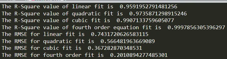
For the R^2 values calculated it can be seen that the fourth order equation fits the best, the higher the R^2 values , the better the fit .

The RMSE error calculated for the various equations show that the linear curve has the biggest error and the fourth order equation curve the lowest error .

More better fit can be obtained using split polynomial functions.

CONCLUSION :

The best fit obtained is on the fourth order equation. However , split wise polynomial functions will also give better fits.