Week 10 - Simulating Combustion of Natural Gas.

Aim- To simulate combustion of natural gas

Objective-

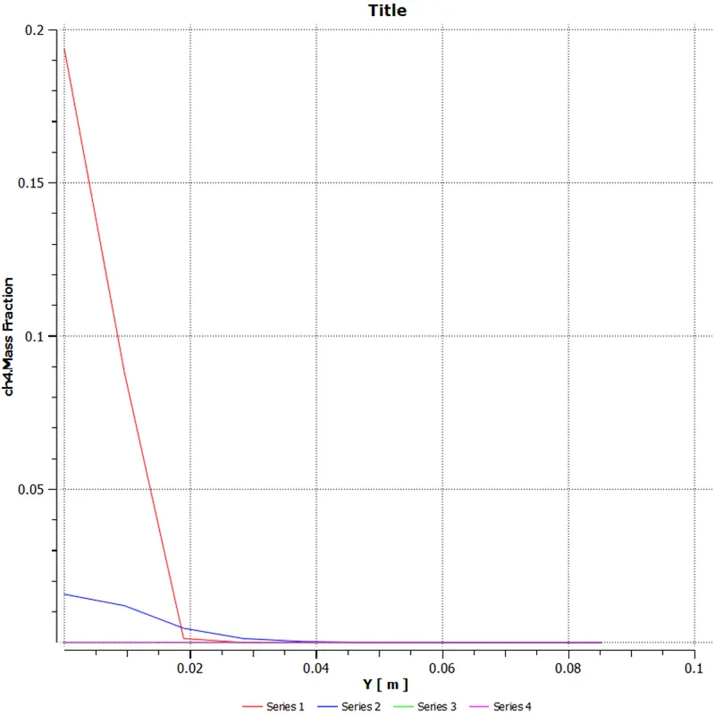
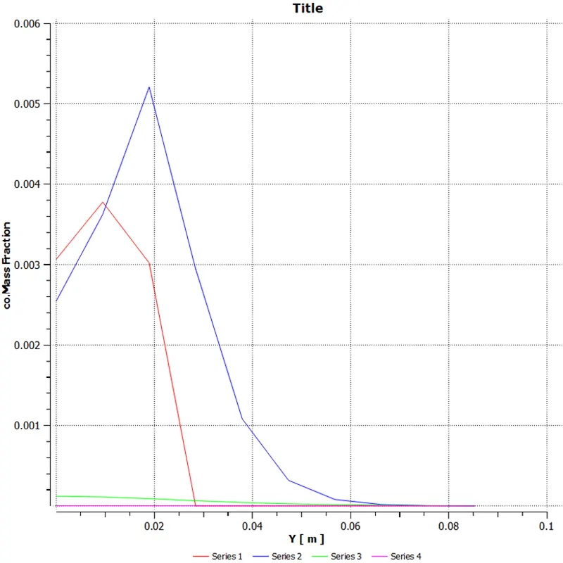
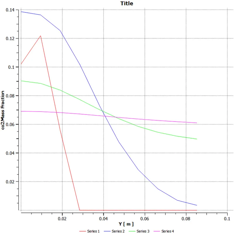
• Perform a combustion simulation on the combustor model and plot the variation of mass fraction of the different species at different locations with using line probes
• In case 2 add water content in the fuel from 5% to 30% by the mole and observe the effect of it on the results

Combustion:

Combustion is a process in which the fuel is oxidized and large amount of chemically bound energy is realised. this energy heats the products and combustion of fuel such as methane with air leads to a flame temperature of around 1900 degree Celsius. In the combustion of methane and air, the Main products are carbon-dioxide and water. However, the formation of this products is very complex and thousands of species such as H, O, OH, CH, CH4 etc are intermediated in the combustion process. The efficiency of combustion process depends on several parameters, such as oxygen supply, temperature and mixing properties

Types of Combustion Simulation:

Based on Mixing

• Non premixed combustion: this type of combustion occurs when oxidizer and fuel mixture enter the reaction zone in distinct streams or not initially mixed. Example of diesel engine where the fuel is injected just before the combustion
• Pre-mixed combustion-the fuel and oxidizer are mixed at molecular level before the combustion similar to case in carburettor
• Partially pre-mixed- its in between non-pre-mixed and premixed combustion where the fuel and oxidizer are partially pre-mixed at non-uniform ratios before combustions

Based on phase

• Fluid phase (volumetric)-this type of combustion occur in fluid phase
• Wall (Surface Reaction)- combustion occurring on surface wall
• Particle (Surface Reaction)-combustion occurs on a surface particle e.g., coal combustion
• Porous-Combustion occurring in a porous region

In this simulation following steps are involved

Geometry

Mesh

Setup

Solution

Results

Geometry

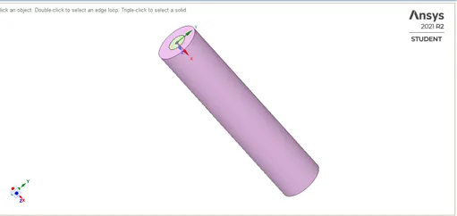
• The 3d model is imported in space claim
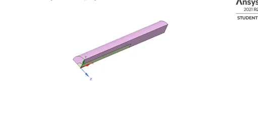
• Use split body command to split the combustor by using cut plane
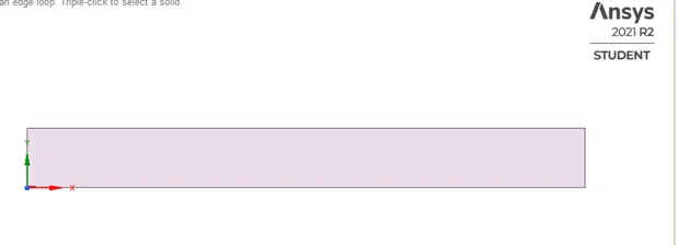
• Now face is copied and created 2 D geometry
• Then use combine command in the space-claim and create final geometry for simulations

Meshing

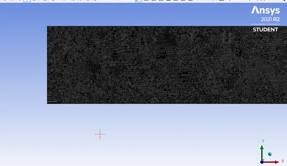
• 2d model is imported for meshing give following parameter for mesh
• Element size=1 mm
• Number of elements=143936
• Number of nodes=72868
• Capture Proximity -yes
• Number of cells across gap=3

Note-give proper named selection for further selections

Setup

• Open fluent setup

General

• Slover-pressure based
• Velocity formulation=Absolute
• Time-Steady
• 2D Space- axis symmetric
• Method=coupled

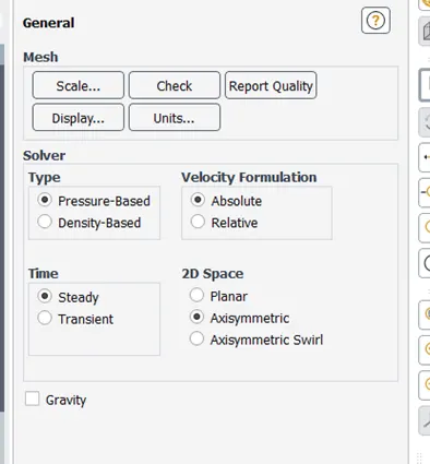
• Energy- turn on

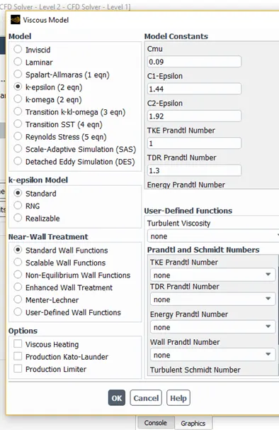
Viscous model

• Model- K epsilon- standard-standard wall function

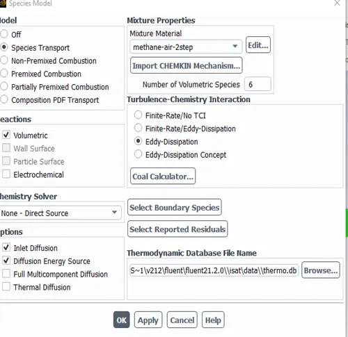
Species

• Model- species Transport
• Mixture material= methane-air-2step
• Turbulence chemistry interaction-eddy dissipation
• Reactions-volumetric

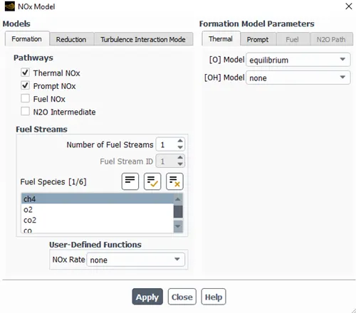
NOx model setting

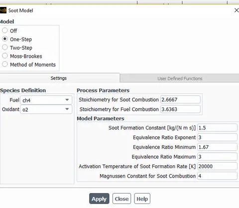
Soot Model

• Model-one step

Boundary condition

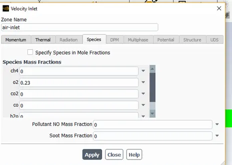
Air inlet-velocity inlet

• Velocity=0.5 m/s
• Temperature=300k
• Species setting- species mass fraction o2=0.23

Fuel-inlet-velocity inlet

• Velocity=80m/s
• Temperature=300k

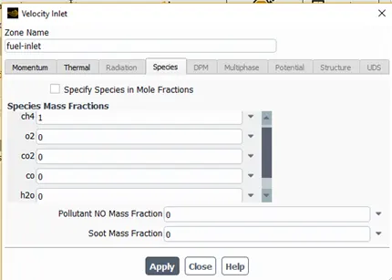
Species setting - species mass fraction CH4=1, H2O=0

Note =for fuel inlet species setting is change according to water content

Solutions

Case 1

Species of mass fractions

CH=1

H2O=0

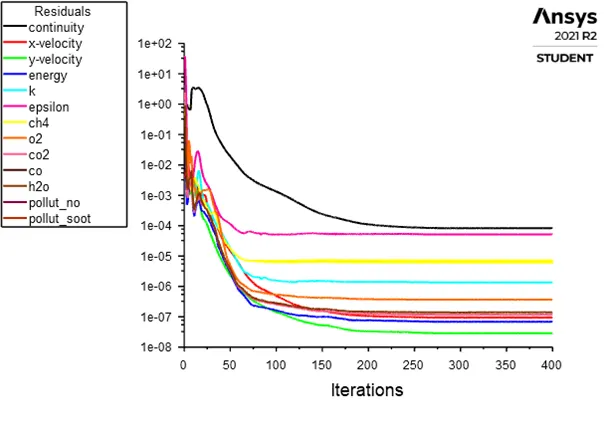
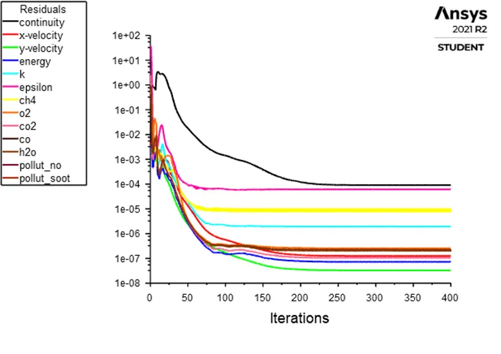
• Residual-solution is run for 400 iterations. from residual plot we can say that our solution is converged after 200-250 iteration because there is no any change in residual plot

Contours

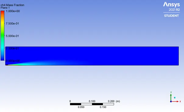
• CH4 Mass Fraction

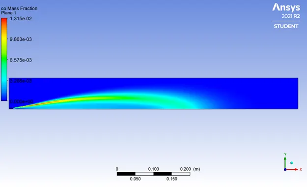
• CO Mass Fraction

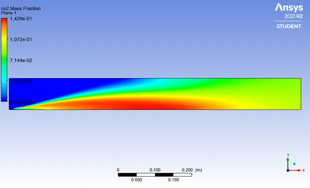
• Co2 Mass Fraction

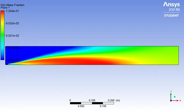
• H2o Mass fraction

• N2 Mass Fraction

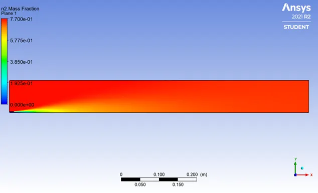
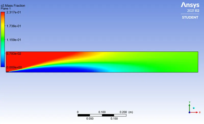
• O2 mass fraction

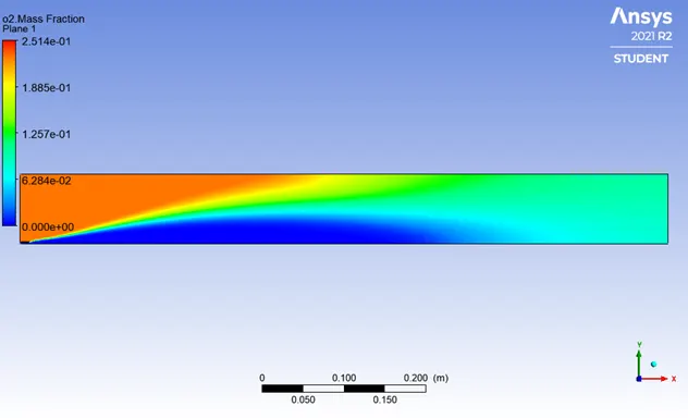
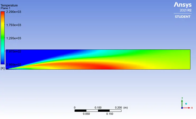
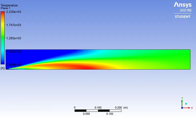
• Temperature contour

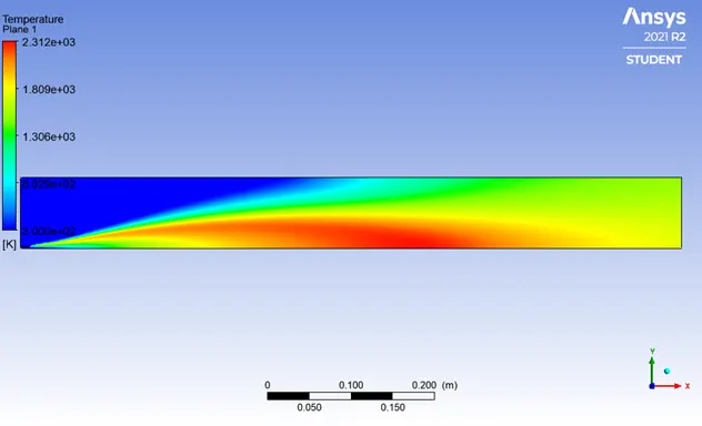
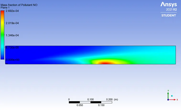
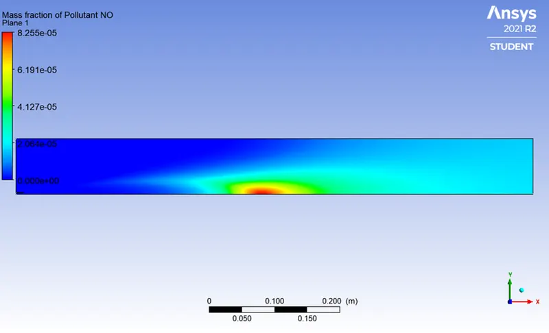
• Mass Fraction of pollutant NO

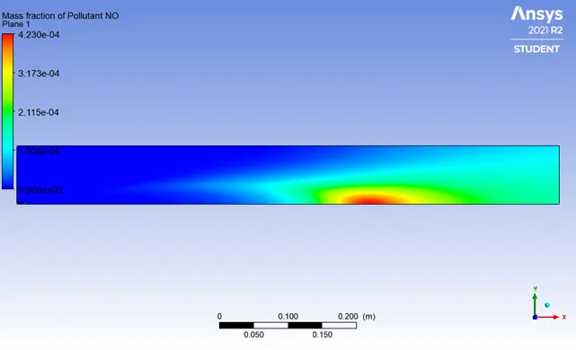
• Mass Fraction of Soot

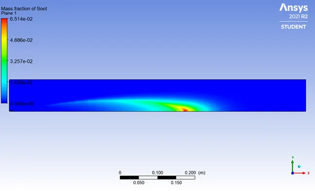
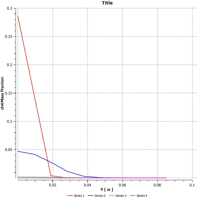
Chart at different location with using line probe

• CH4 Mass Fraction

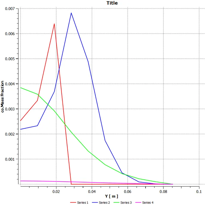
• Co Mass Fraction

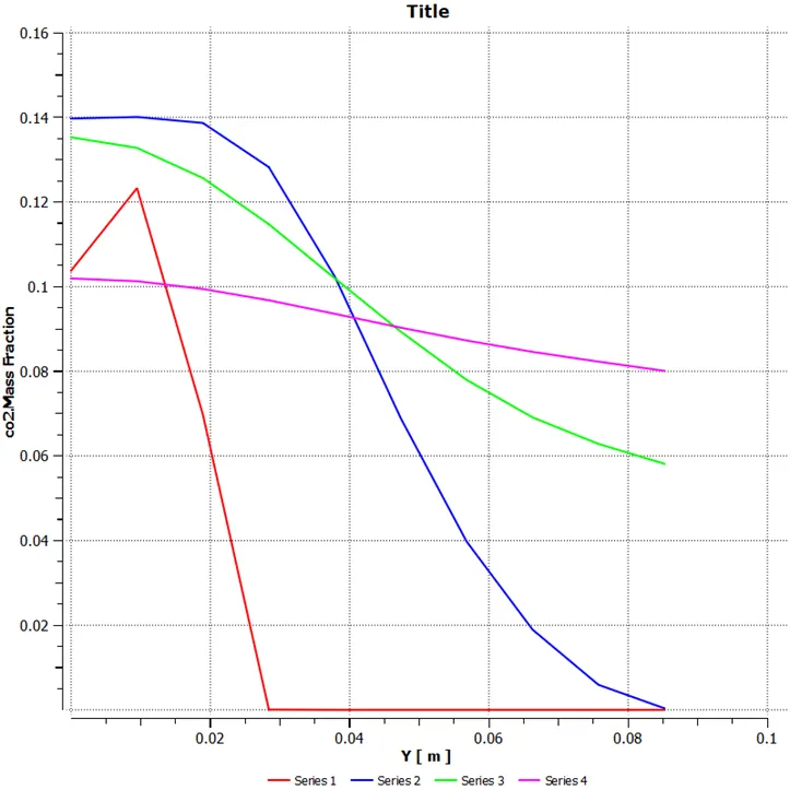
• CO2 mass fraction

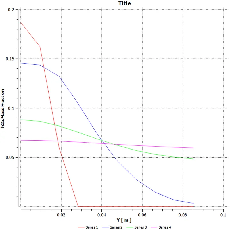
• H2O mass fraction

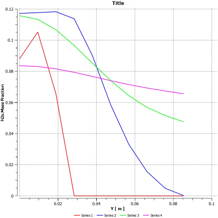
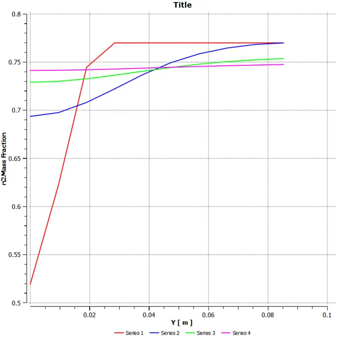
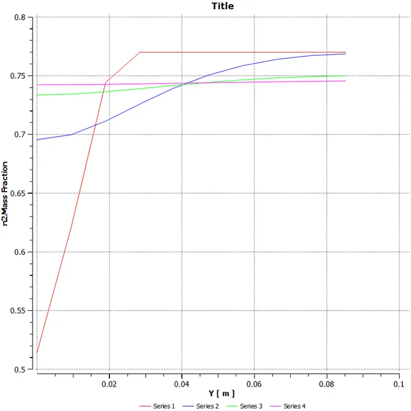
• N2 mass fraction

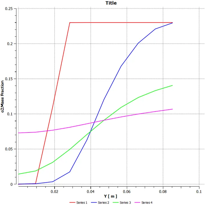
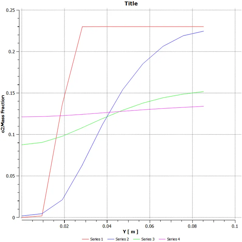
• O2 mass fraction

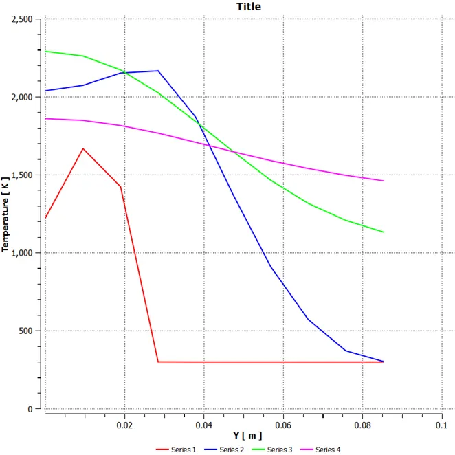
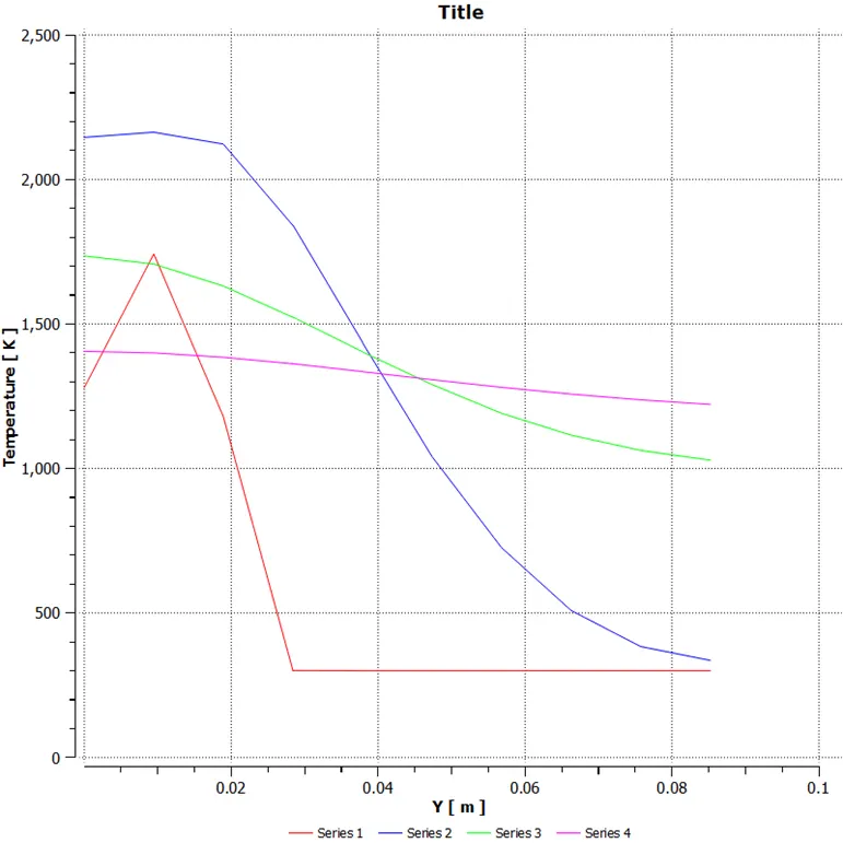
• Temperature chart

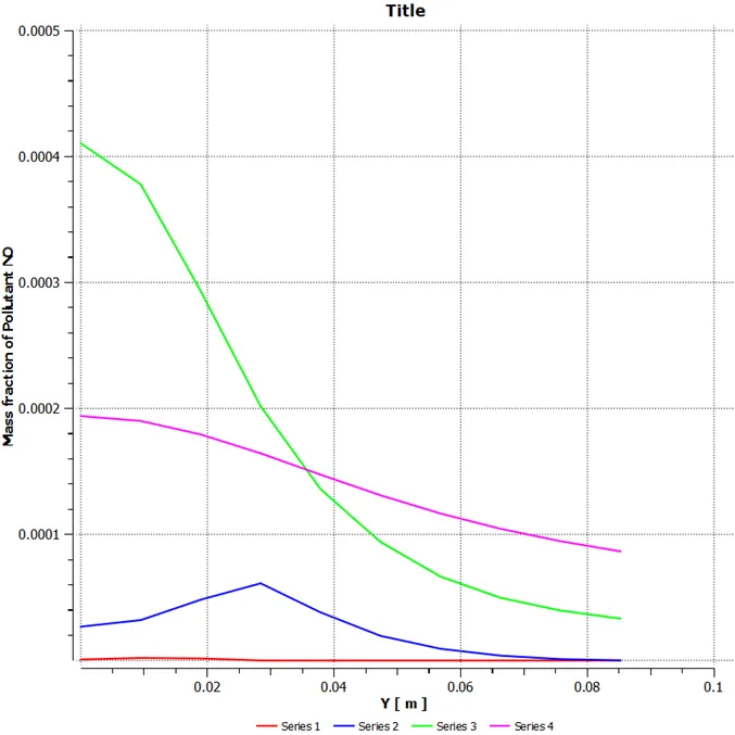
• Mass Fraction of pollutant NO

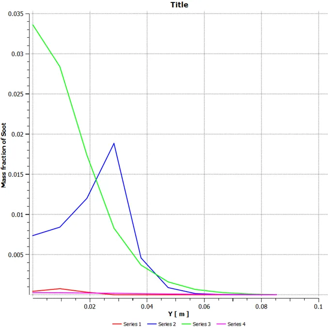
• Mass Fraction of soot

Species of mass fractions

CH=0.95

H2O=0.05

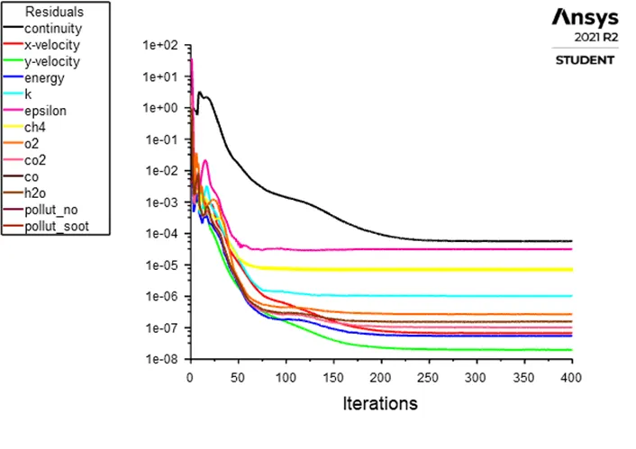
• Residual-solution is run for 400 iterations. from residual plot we can say that our solution is converged after 200-250 iteration because there is no any change in residual plot

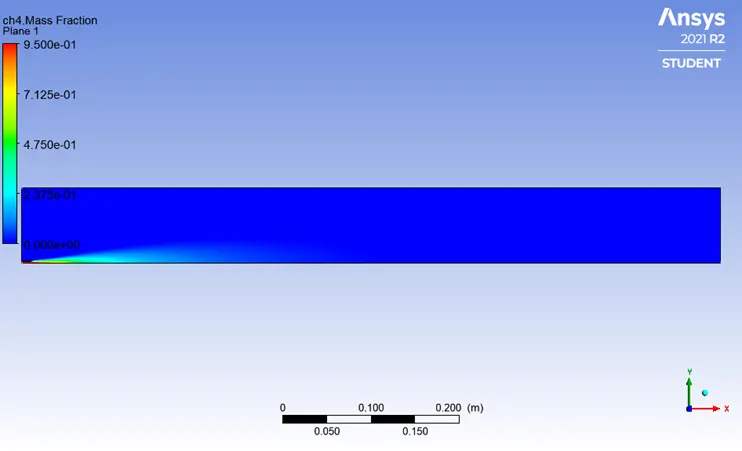
• CH4 Mass Fraction

• Co mass fraction

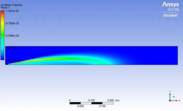
• Co2 Mass fraction

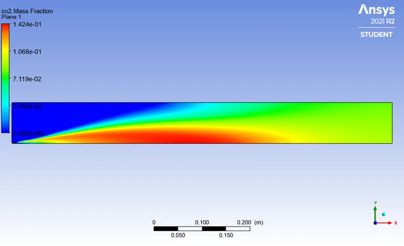
• H20 Mass Fraction

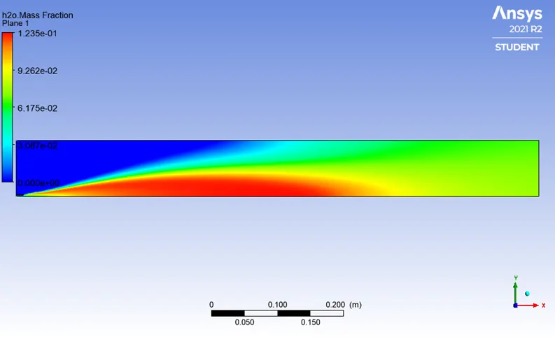
• N2 mass fraction

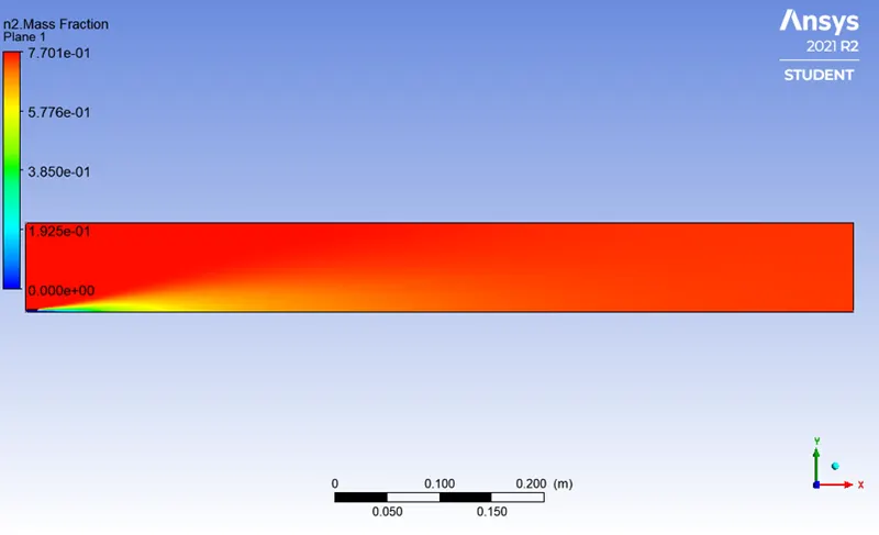
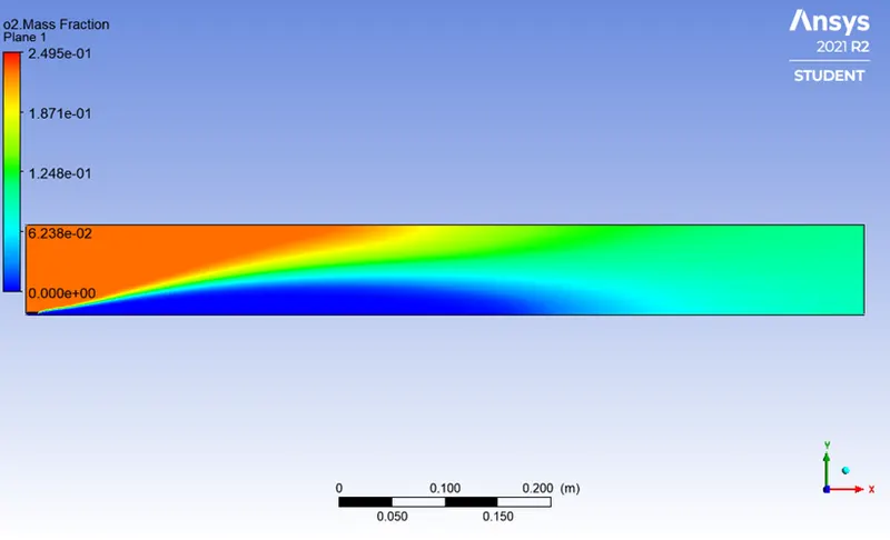
• O2 mass fraction

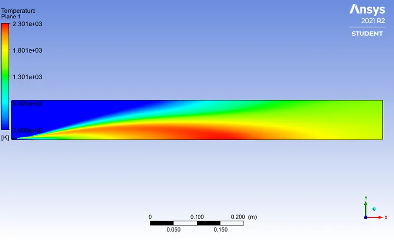
• Temperature contour

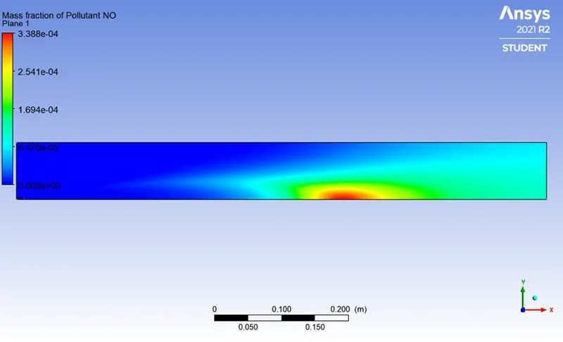
• Mass fraction of pollutant NO

• Mass Fraction of soot

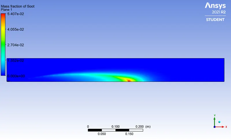
Chart at different location with using line probe

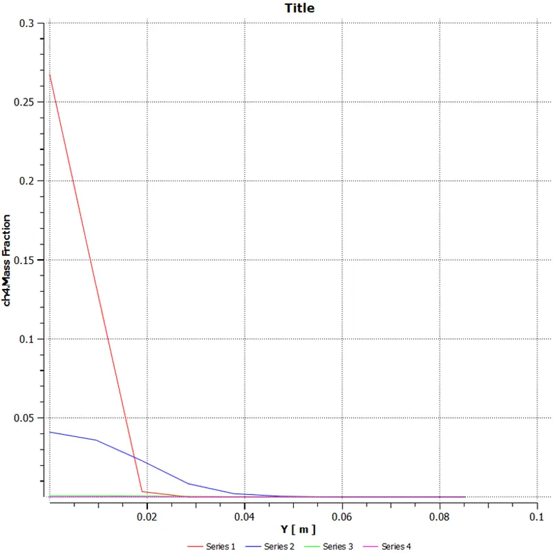
• CH4 mass fraction

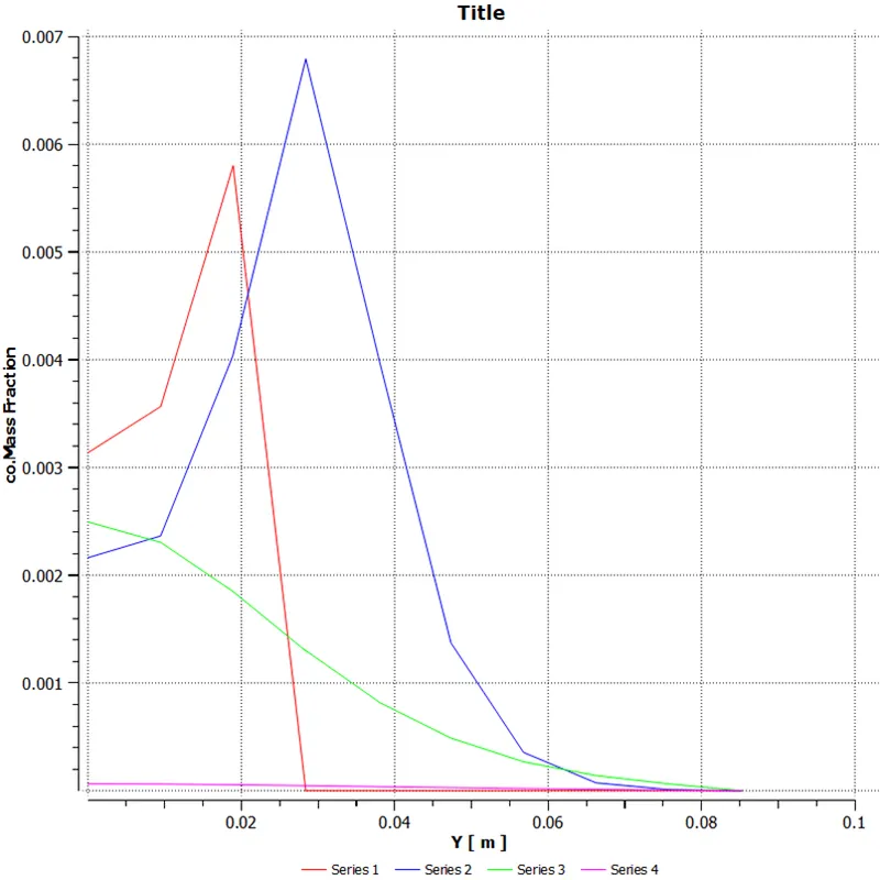
• Co Mass fraction

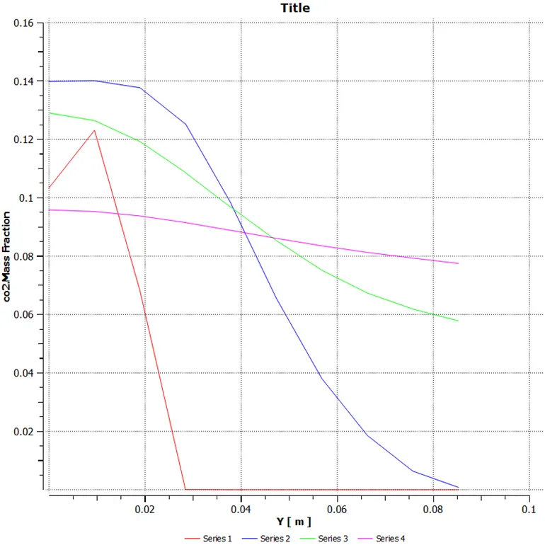
• Co2 Mass Fraction

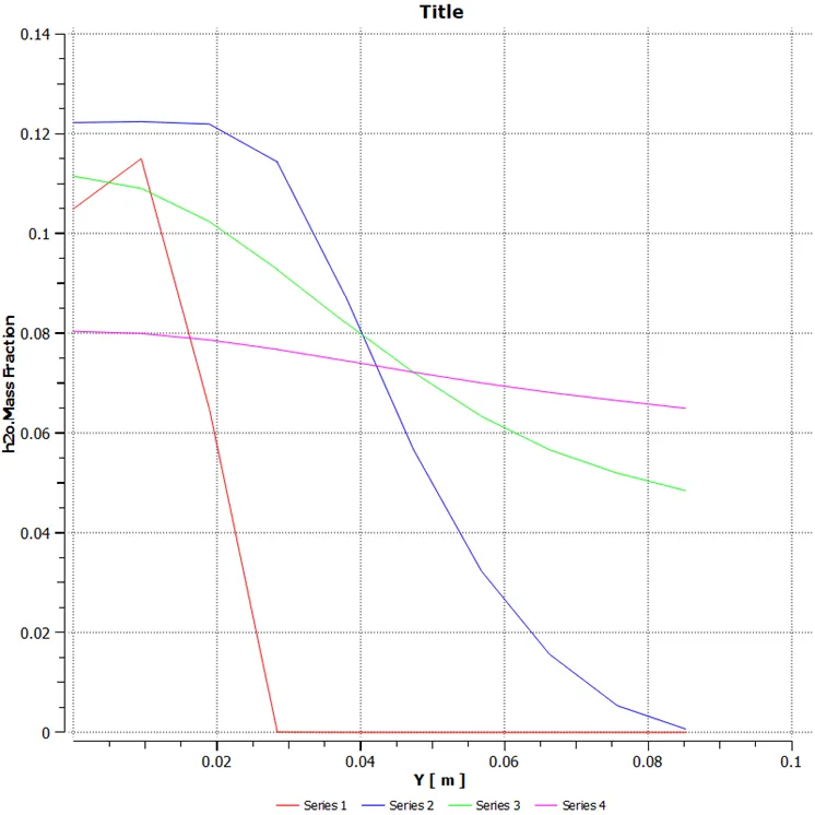
• H2o Mass Fraction

• N2 mass fraction

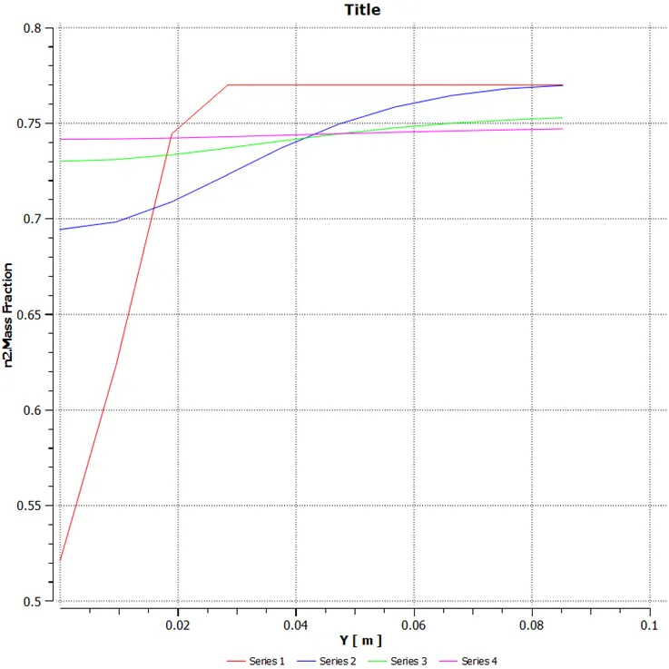
• O2 Mass fraction

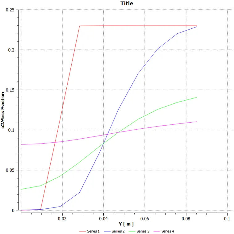
• Temperature Chart

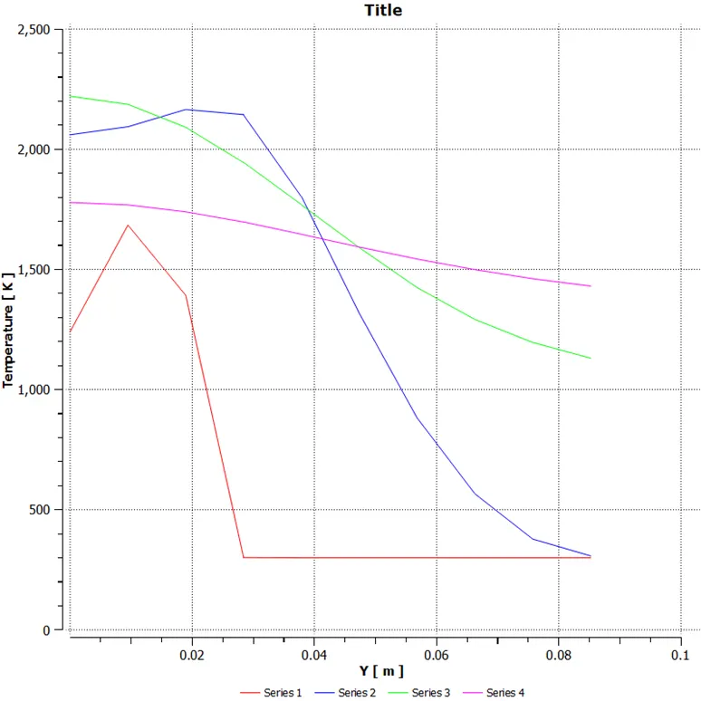
• Mass fraction of pollutant NO

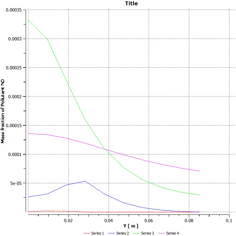
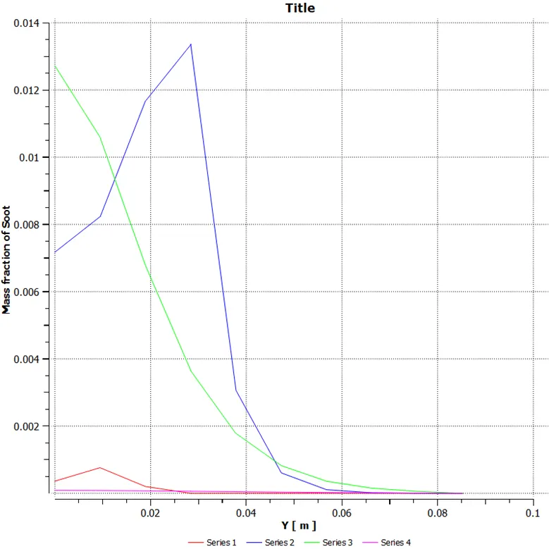
• Mass Fraction of Soot

Species of mass fractions

CH=0.9

H2O=0.1

• Residual-solution is run for 400 iterations. from residual plot we can say that our solution is converged after 200-250 iteration because there is no any change in residual plot

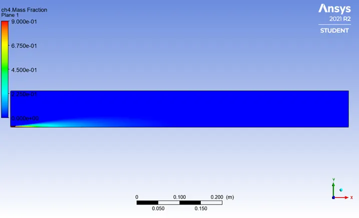
• Ch4 Mass fraction

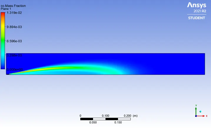
• Co mass fraction

• Co2 Mass fraction

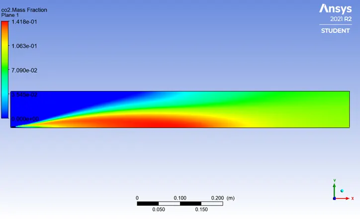
• H2o mass fraction

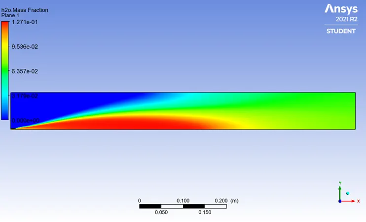
• N2 mass fraction

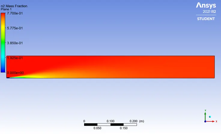
• O2 mass fraction

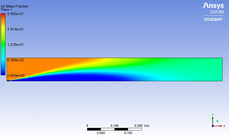
• Temperature contour

• Mass fraction of pollutant NO

• Mass fraction of soot

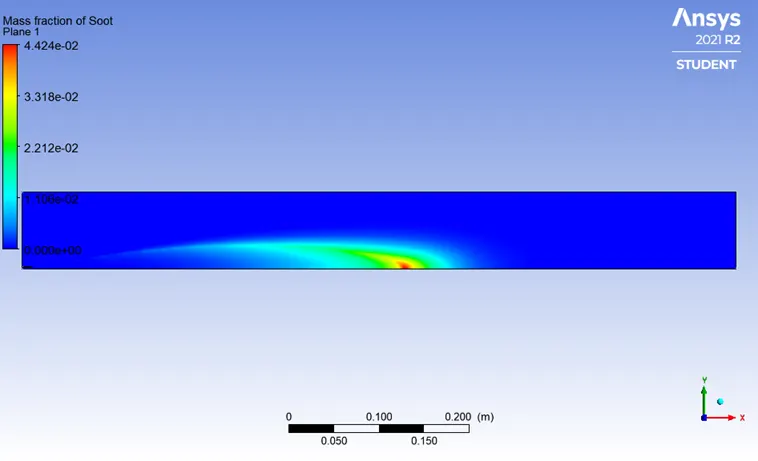
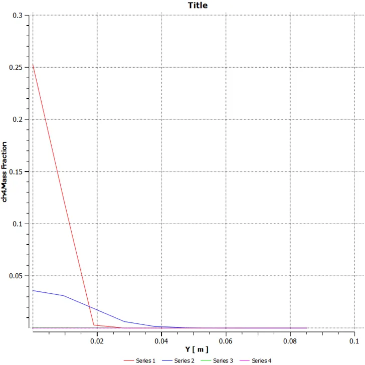
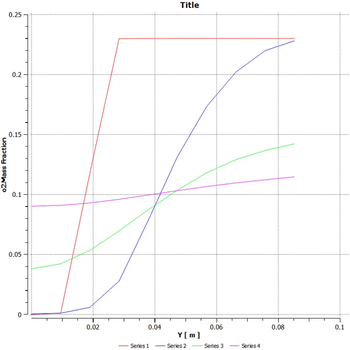
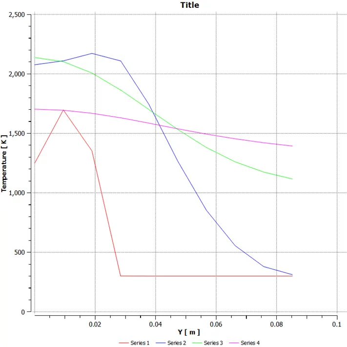
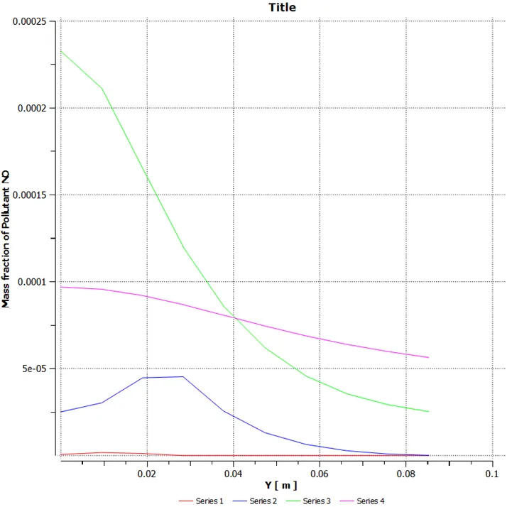
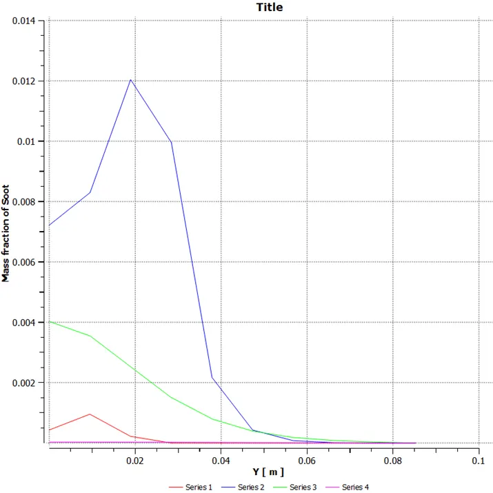
Chart at different location with using line probe

• CH4 mass fraction

• Co mass fraction

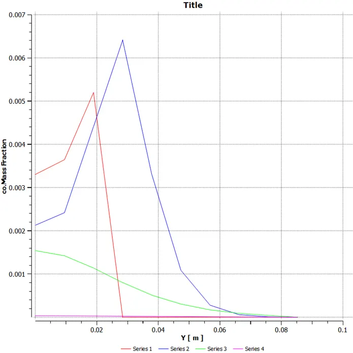
• Co2 mass fraction

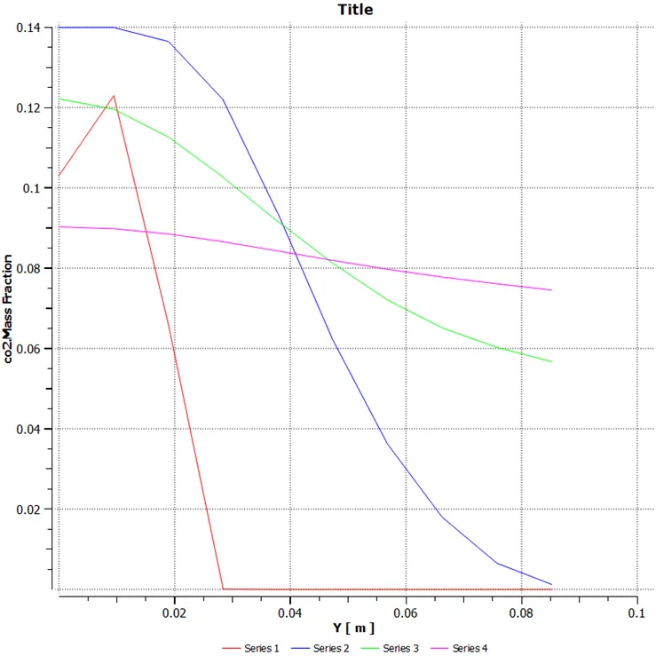
• H2o mass fraction

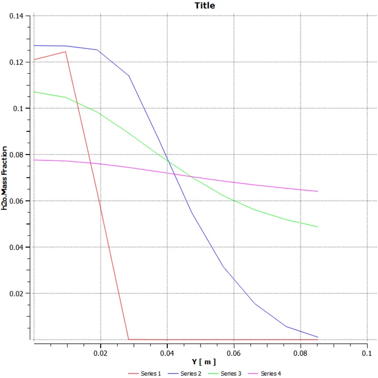
• N2 mass fraction

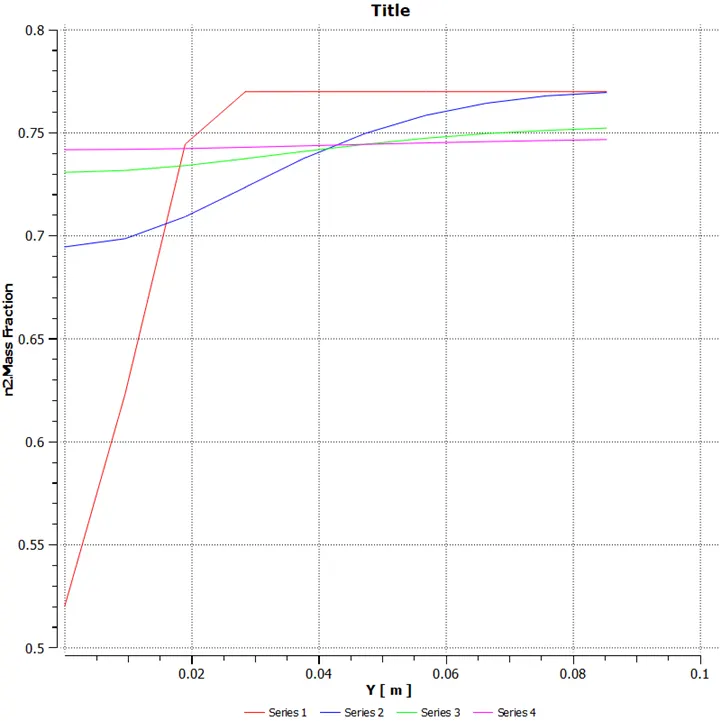
• O2 Mass fraction

• Temperature chart

• Mass fraction of pollutant NO

• Mass fraction of Soot

Species of mass fractions

CH=0.8

H2O=0.2

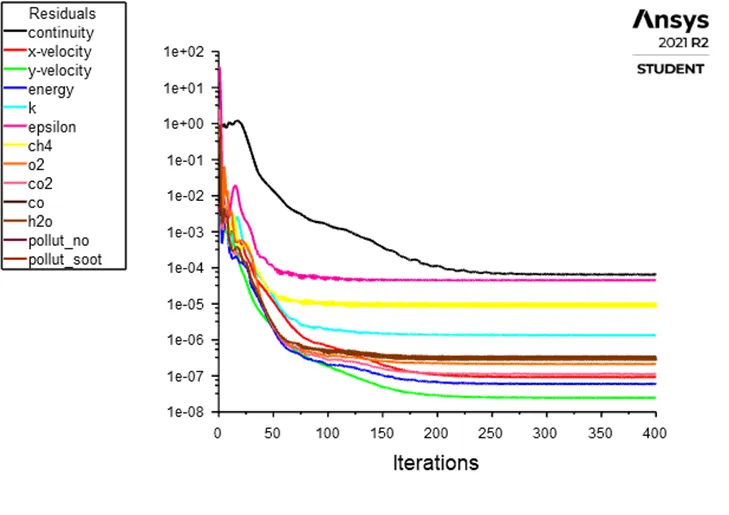
• Residual-solution is run for 400 iterations. from residual plot we can say that our solution is converged after 200-250 iteration because there is no any change in residual plot

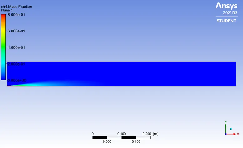
• CH4 Mass Fraction

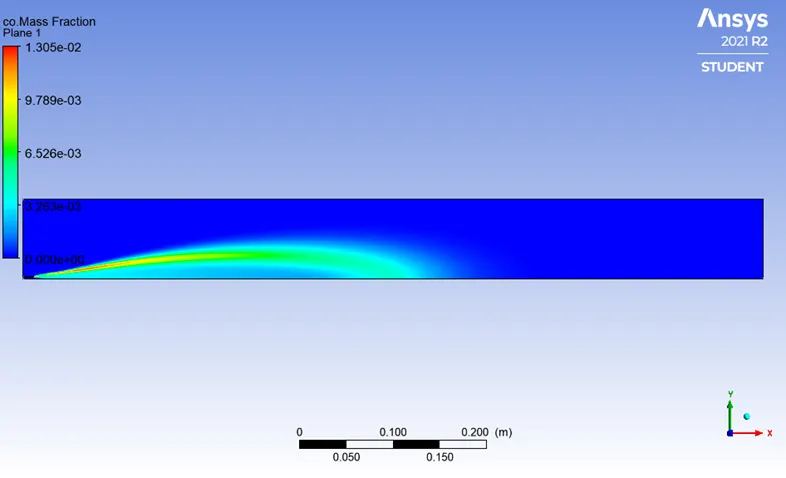
• Co mass Fraction

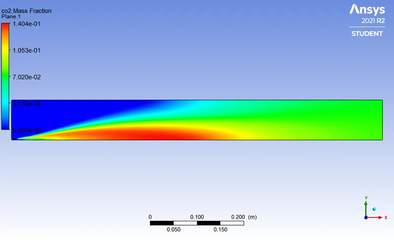
• Co2 Mass Fraction

• H2o mass fraction

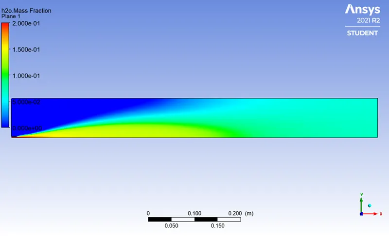
• N2 mass fraction

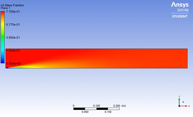
• O2 mass fraction

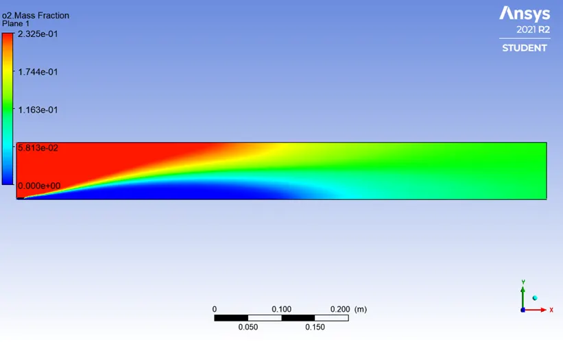
• Temperature contour

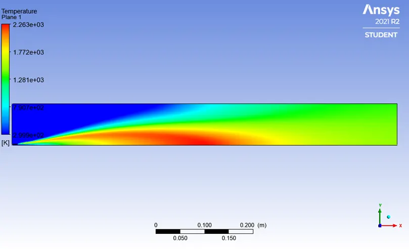
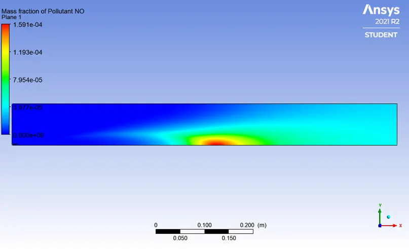
• Mass fraction of pollutant NO

• Mass Fraction of soot

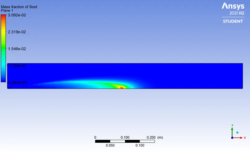
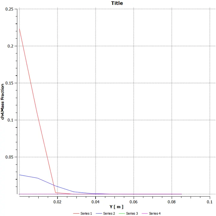
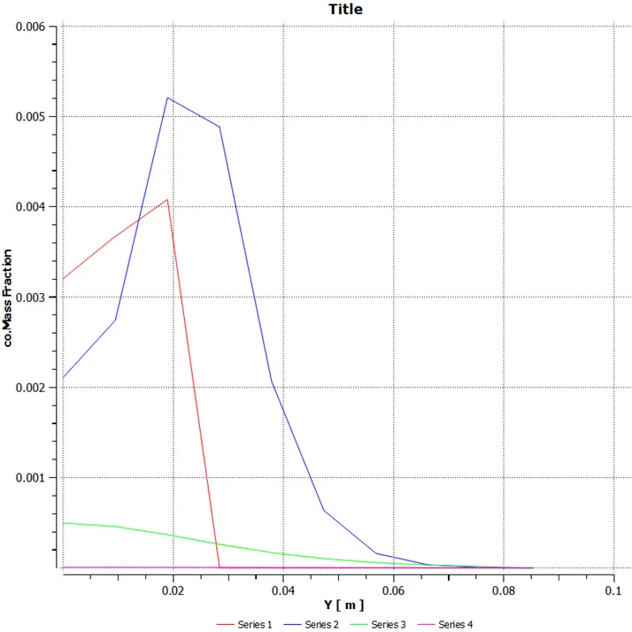
Chart at different location with using line probe

• CH4 mass fraction

• CO mass fraction

• CO2 mass fraction

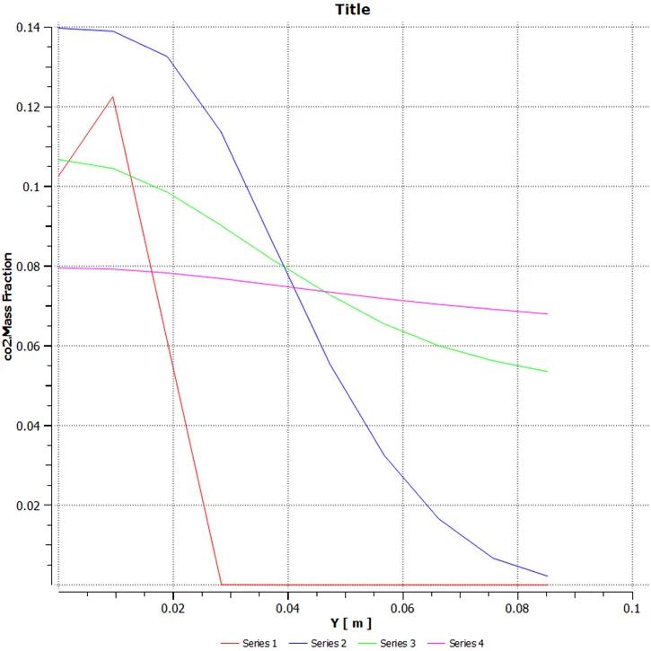
• H2o mass fraction

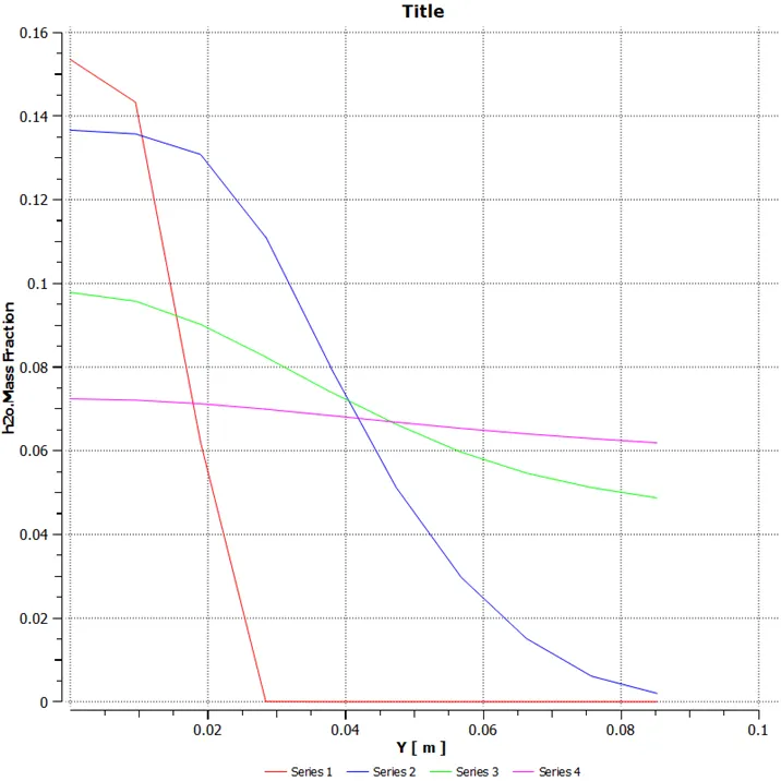
• N2 mass fraction

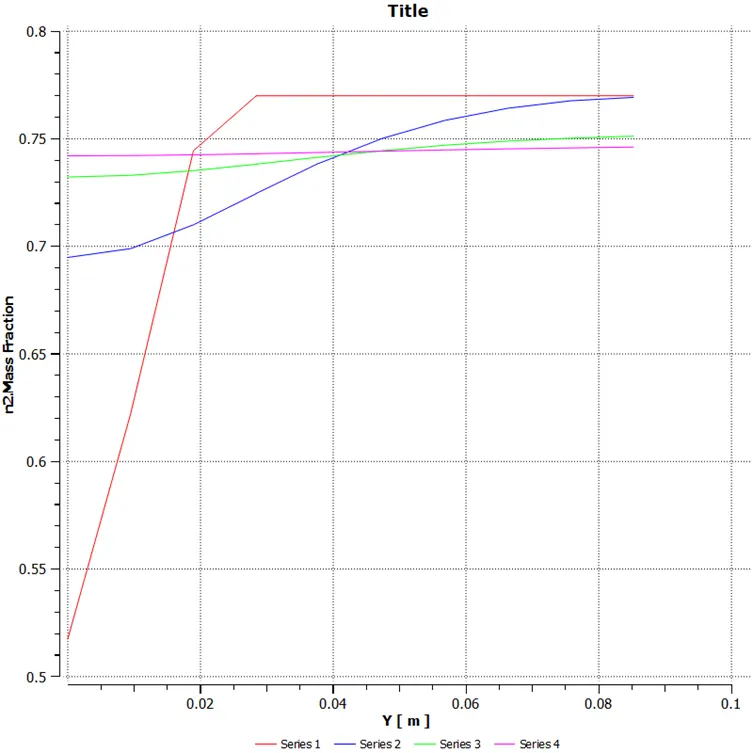
• O2 mass fraction

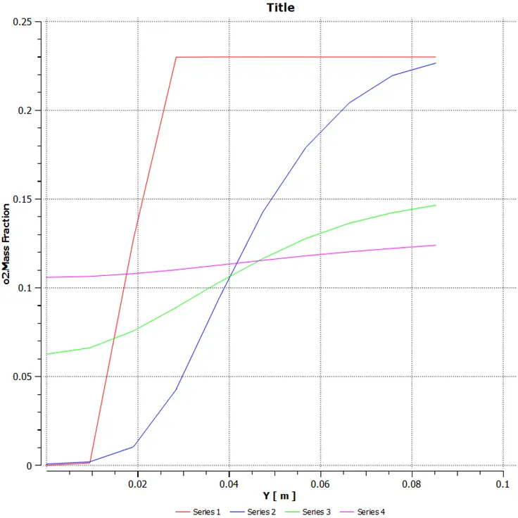
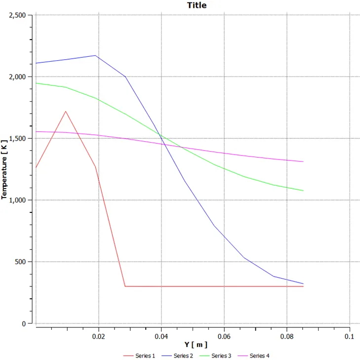
• Temperature chart

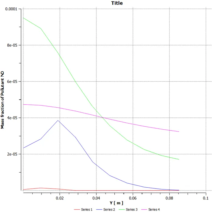
• Mass Fraction Of Pollutant NO

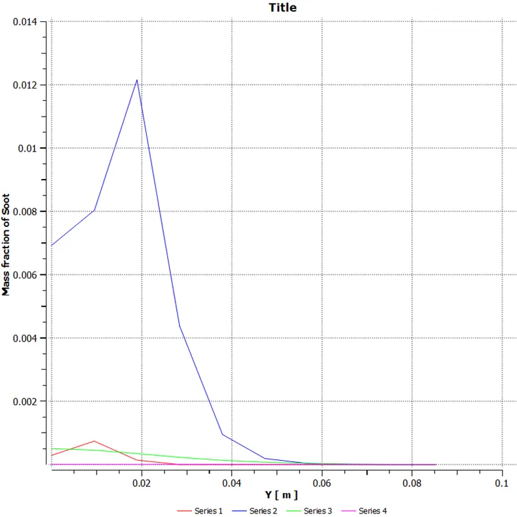
• Mass fraction of soot

Species of mass fractions

CH=0.7

H2O=0.3

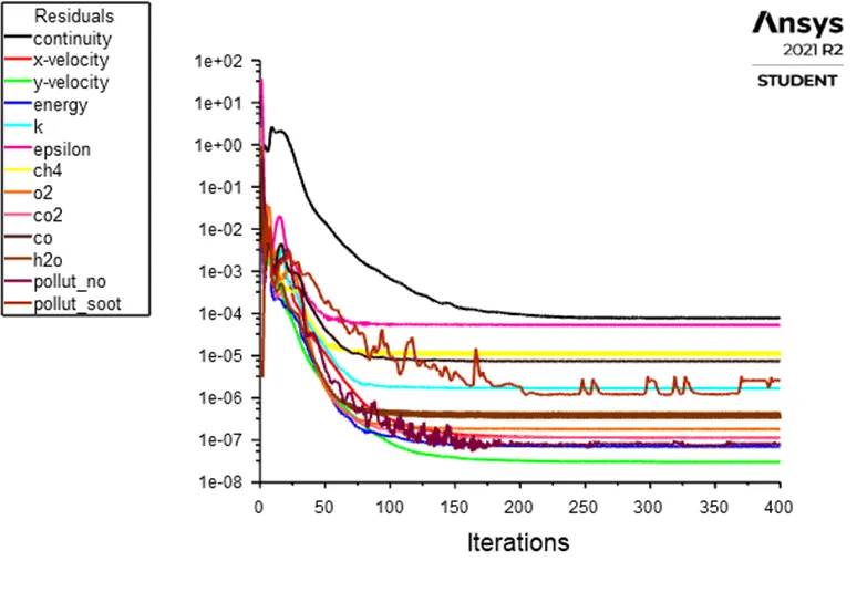
• Residual-solution is run for 400 iterations. from residual plot we can say that our solution is converged after 150-200 iteration because there is no any change in residual plot

• CH4 mass fraction

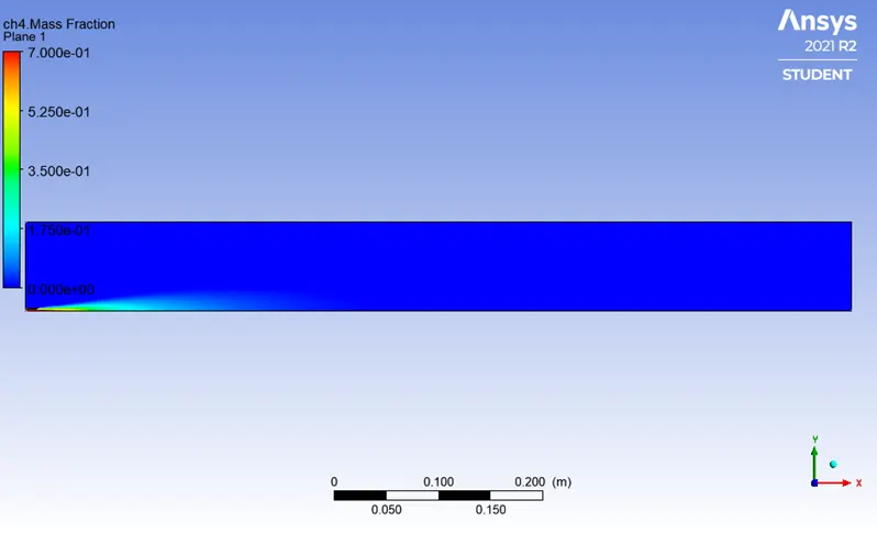
• Co mass fraction

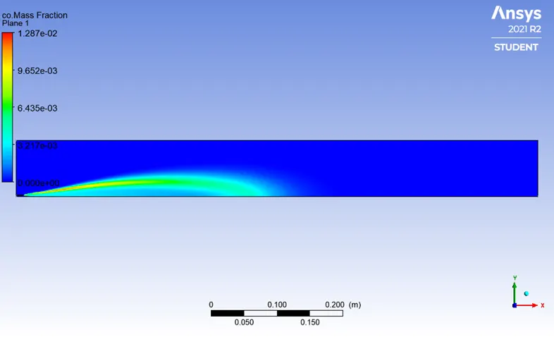
• Co2 mass fraction

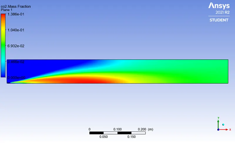
• H2O Mass fraction

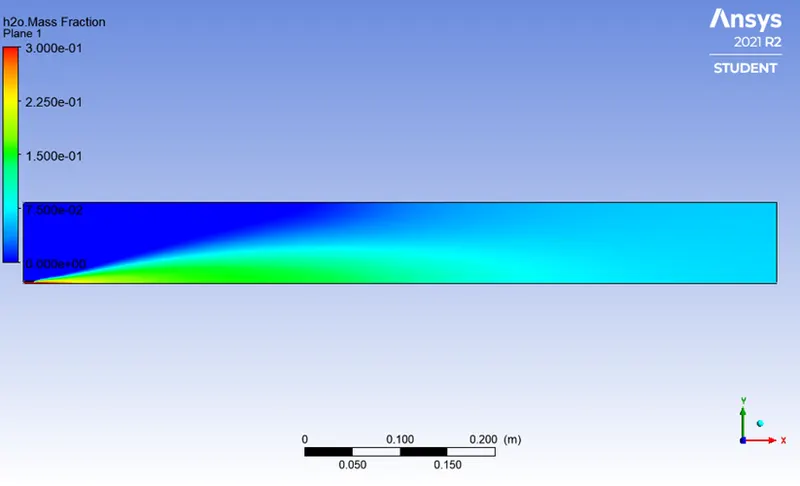
• N2 Mass fraction

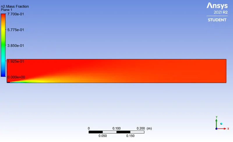
• O2 Mass fraction

• Temperature contour

• Mass fraction of pollutant NO

• Mass fraction of soot

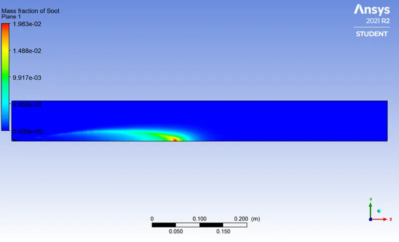
Chart at different location with using line probe

• CH4 mass fraction

• Co mass fraction

• Co2 mass fraction

• H2o mass fraction

• N2 Mass fraction

• O2 Mass Fraction

• Temperature chart

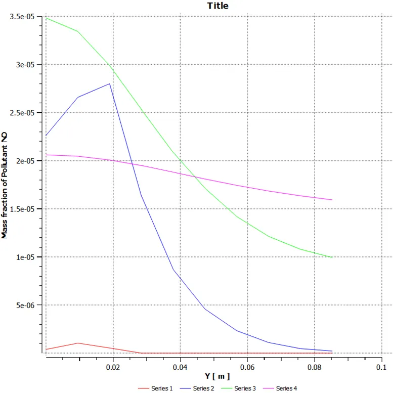
• Mass fraction of pollutant NO

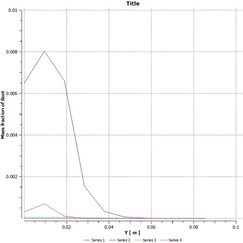
• Mass fraction of soot

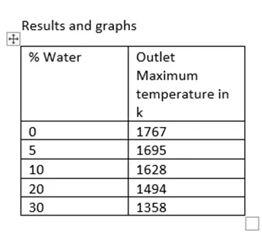
Results and graphs

Table: Outlet temperature

Outlet maximum temperature vs % water

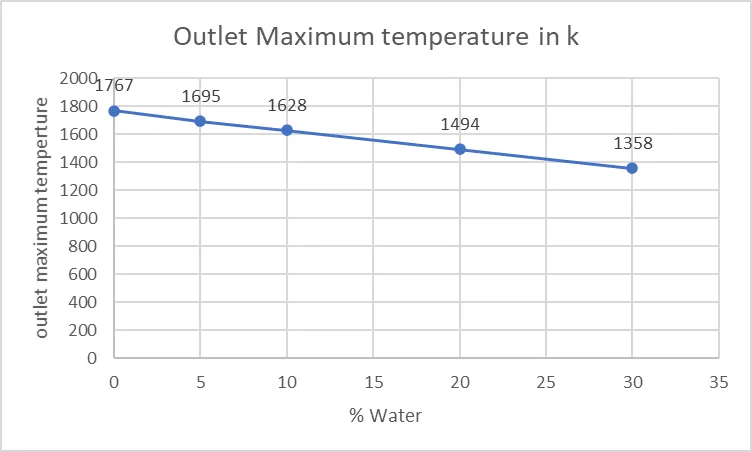
Table: Mass fraction of soot

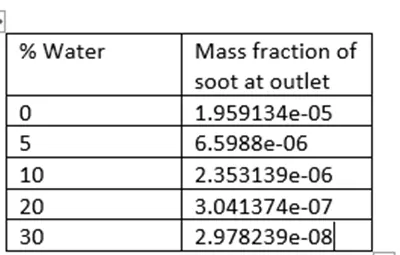
Mass fraction of soot at outlet vs % Water

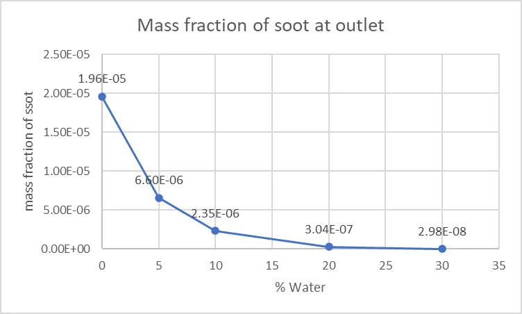
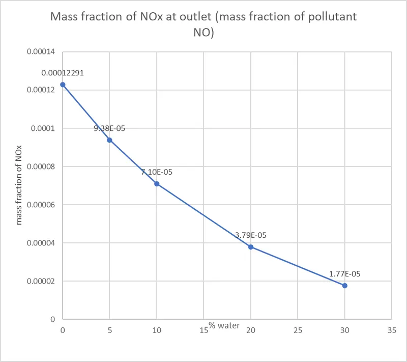
Table: Mass fraction of NOx (mass fraction of pollutant NO)

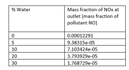
Mass fraction of NOx at outlet vs % Water

Conclusion-

• Simulation is done at changing the % water content and observe the changes for each case after increasing % water content
• Plot the graph of mass friction of soot and mass friction of NOx against % water content and observe the results
• Maximum temperature at outlet decreases with increasing % of water content
• Mass fraction of soot at outlet is decreased with increasing % of water content
• Mass fraction of NOx at outlet is decreased with increasing % of water content