Week 10 - Simulating Combustion of Natural Gas.
Aim
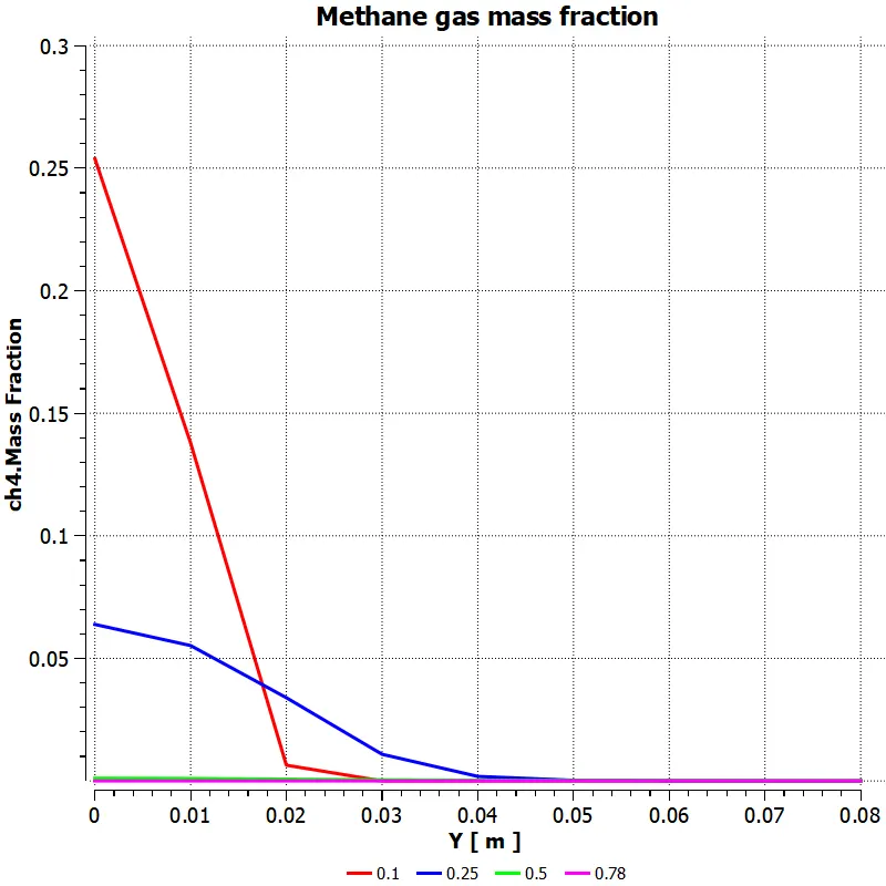
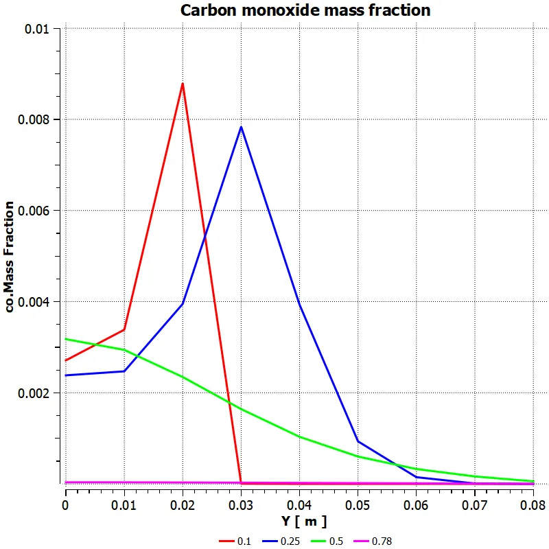
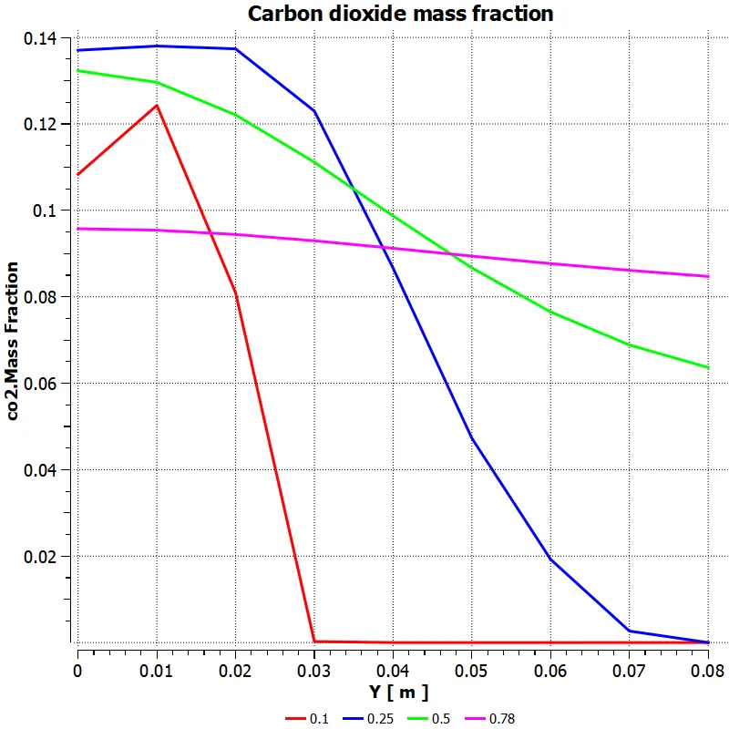
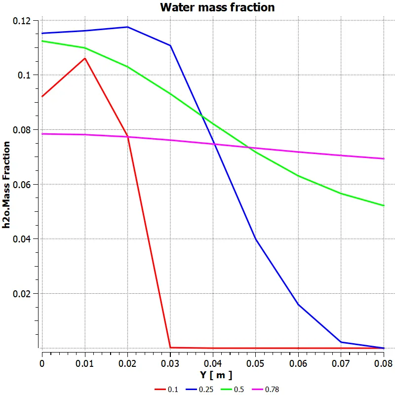
- Perform a combustion simulation on the combustor model and plot the variation of the mass fraction of the different species’ in the simulation using line probes at different locations of the combustor as shown in Fig. You need to plot for CO2, H2O, CH4, N2, O2, NOx emissions & Soot formation.
- As a second part, we have to add the water content in the fuel from 5% to 30% by mole and observe the effect of it on the results.
Introduction
Natural gas combustion is an exothermic chemical reaction in which natural gas and oxygen react, producing heat and several chemical byproducts. This reaction can be controlled and harnessed to generate heat for cooking and heating. It can also be used to power an electrical generator used to create electricity which can be used for lighting and other purposes. Natural gas is comprised primarily of methane. Sources for natural gas include fossil fuel deposits which can be processed to yield natural gas and biofuel generators which can be used to make methane from biological material. The gas is treated to make it as pure as possible, removing compounds which could impair the combustion process or generate pollution which would make combustion harmful to the environment.
In the past years strategies for the reduction in soot emissions relied mainly on correlations, experience and trial-and-error attempts. The increasingly diffusion of CFD is allowing to analyze and optimize combustion devices with sufficient confidence. However, the uncertainty increases significantly when soot is concerned: the complexity of the gas-phase chemistry and the numerous mechanisms involved in soot formation process, which are strongly coupled with mixing and radiative heat transfer and depend on soot volume fraction itself, make the prediction of soot emissions still a challenging task, leading to large errors in exhaust concentration even with small mispredictions in the formation rates
Different mechanisms are in fact involved in the determination of the final concentration at the exit of the combustion device, such as inception, coagulation, surface growth and oxidation. Even though reasonable predictions can be achieved on laminar diffusion flames , the scenario is further complicated when turbulent flames burning common fuels such as diesel or kerosene are concerned, as the applicability of models developed for simple aliphatic hydrocarbon fuels (such as methane) is questioned. Soot production in methane-air flames usually takes place from small species (e.g. acetylene) that grow to form polyaromatic hydrocarbons (PAH) and eventually soot.
- Soot is a mass of impure carbon particles resulting from the incomplete combustion of hydrocarbons
Geometry
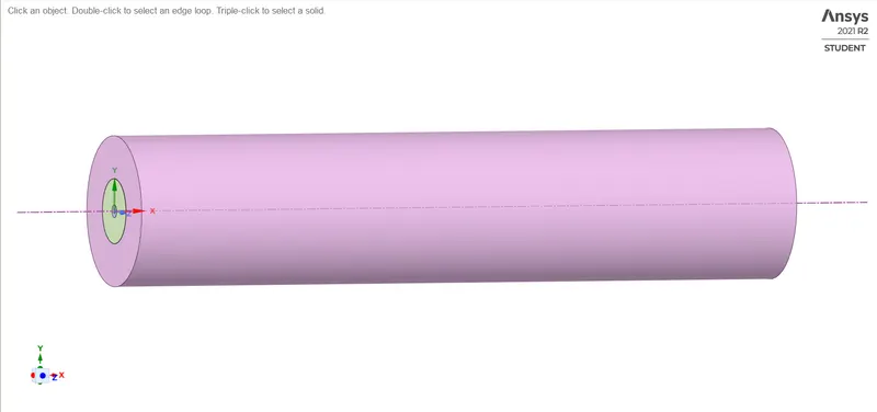
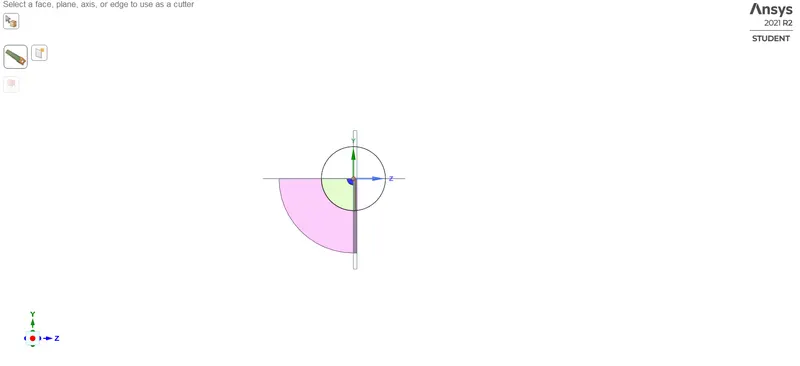
- The 3D geometry is loaded onto the space claim and it is Splitted using 'Split by plane' tool at centre of the Cylinder
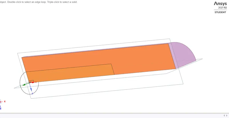
- It is again Split into Respective halves
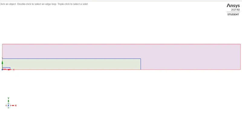
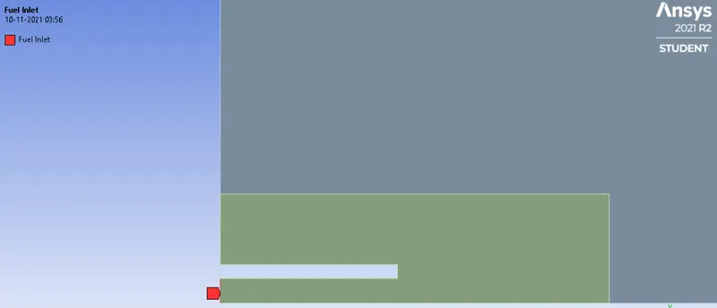
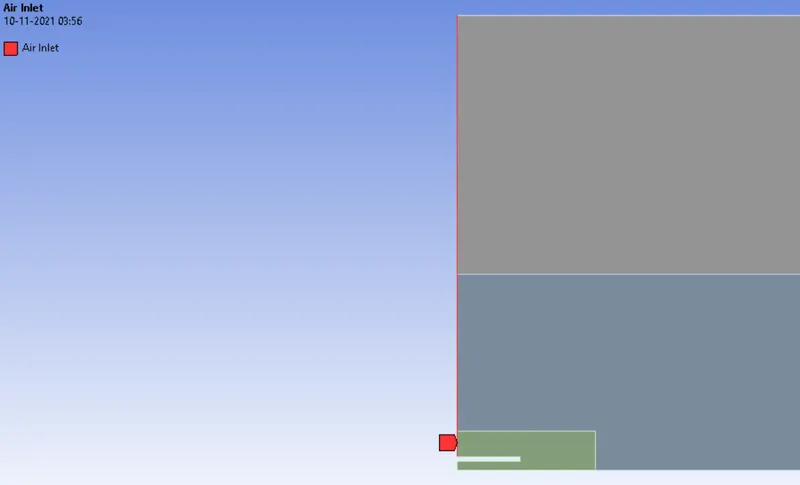
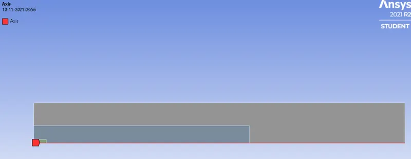
- One face is copied representing the 2D image of the cylinder as shown in the pictures
- The copied face it pasted on to a new spaceclaim and the whole face is selected and Share topology is enabled to enable the interaction between the cylinders
- Cylinders of different sizes is used here to mesh the respective zones effectively
Mesh
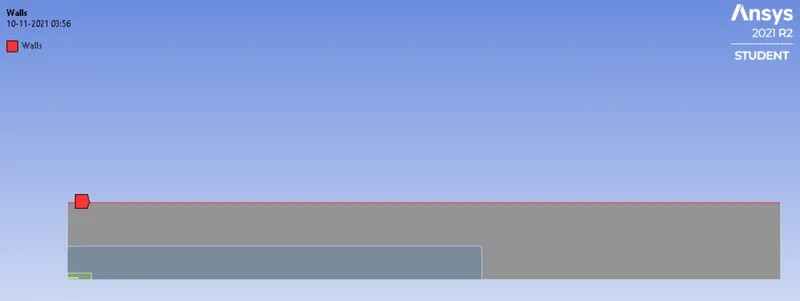
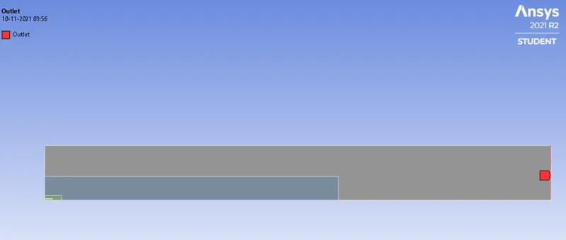
- Named selection is added to the edges as shown is the pictures
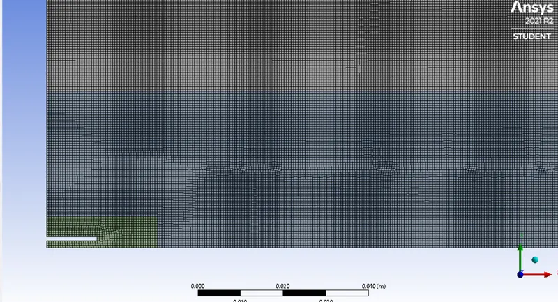
- mesh size of 5e-2m is given to the Outer cylinder
- mesh size of 5e-3m is given to the Middle cylinder
- mesh size of 1e-3m is given to the Inner cylinder
- Capture proximity is turned on with number of cells across gaps as 3
Setup
- Steady state , pressure based and Axis symmetris calculation is selected
- Energy is enabled since the calculation involves temperature terms
- Viscous model is set to K-epsilon
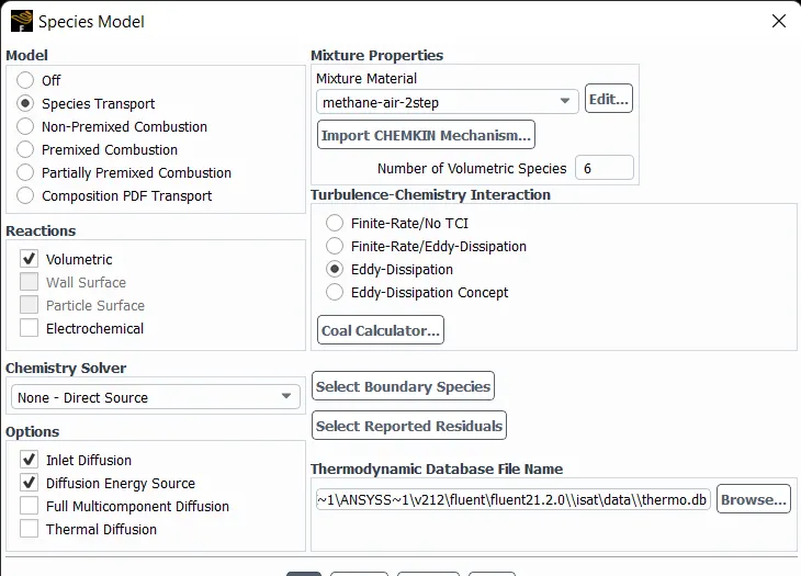
- Species is turned on With species transport equation
- Within the species menu Vomlumetric reaction is selected , Inlet diffusion and Diffusion energy sources are also added
- For species the mixture material is set to Methane-Air-2step to enable the presence of water
- Boundary conditions for Air-Inlet are ,Velocity = 0.5m/s ,Temperature = 300k , Species-> Oxigen with mass fraction 0.23.And for Fuel inlet Velocity is set to 80m/s with Species as 1 mass fraction for CH4 (mathane). The respective mass fractions are calculated as show below
So Since air contains mostly (79% nitrogen and 21% Oxigen )we have the equation for the reactants as `CH_4 + ar(O_2+3.76N_2)` where ar is the stoichiometric coefficient. And we have the product side as `aCO_2+bH_2O+cN_2` ,
we have to balance the product side and reactant side using the coefficients a,b,c
Balancing carbon atoms , a =1.
Balancing Hydrogen atoms , 4=2b `=>`b = 2.
For balancing 'ar' Take the coefficients of oxigen and nitrogen from products side and equate them
hence 2ar = 2a+b
ar =a + b/2
= 1+1 =2
Now we can fine the inlet Mass fractions for Fuel and air
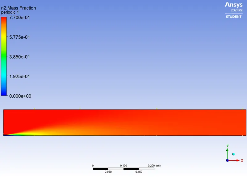
Air contains 2 moles of Oxigen (O2) and 7.52 moles of Nitrogen , The Oxigen Mole fraction would be 2/(2+7.52) = 2/9.52 = 0.21 , when converted to mass fraction it would be 0.23
Since CH4 is only of 1 mole we can Input the fuel inlet with mass fraction of 1 for CH4 in Fuel inlet
- Outlet is Pressure based
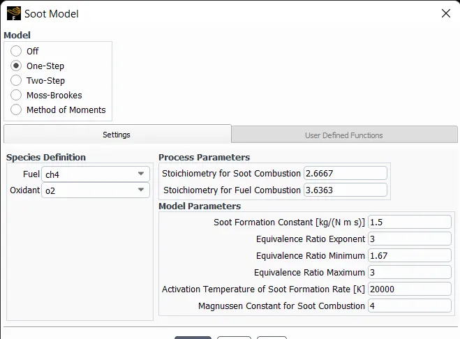
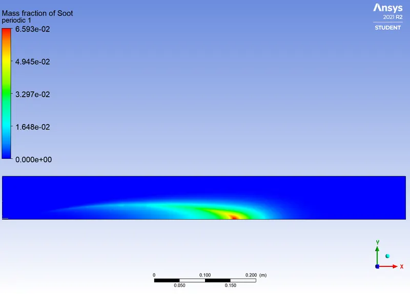
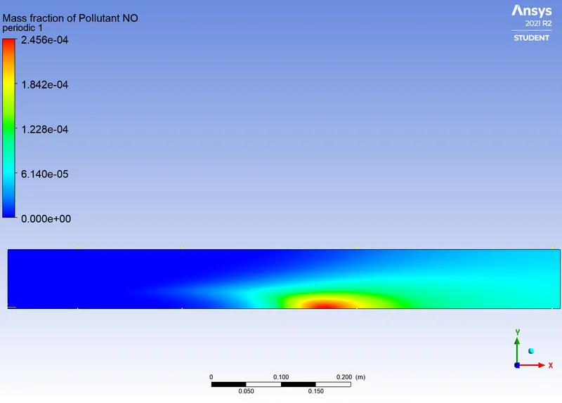
- Inorder to capture the mass fractions Soot and NOx , The respective options under Species is enabled. The Soot model is set to one-step with Fuel as CH4 and oxident as oxigen.
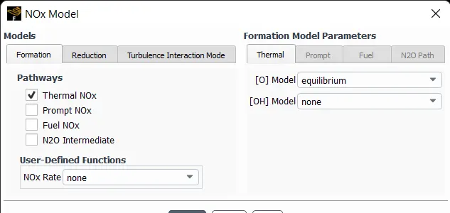
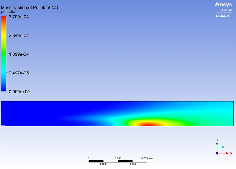
- In Nox model only the Thermal Nox is enabled since major part of this compund is formed during high temperatures
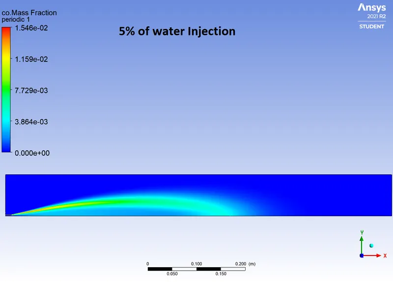
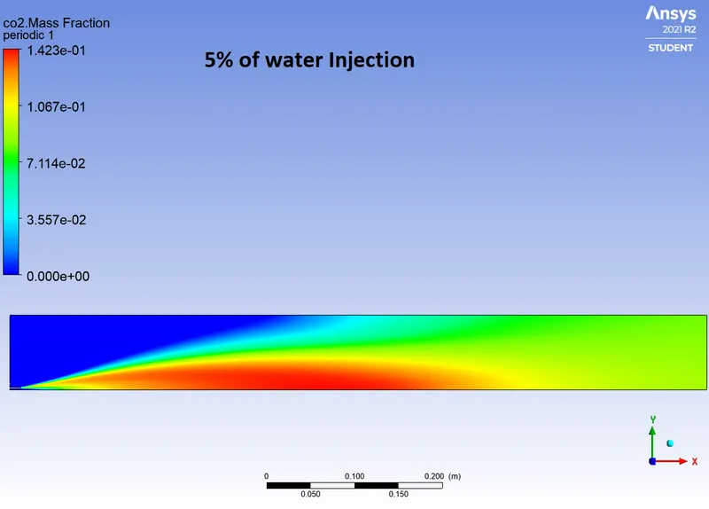
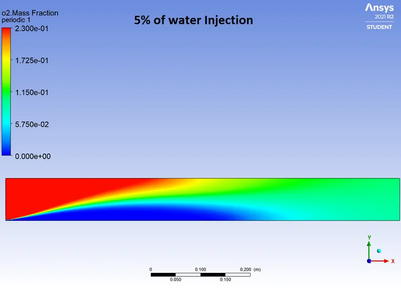
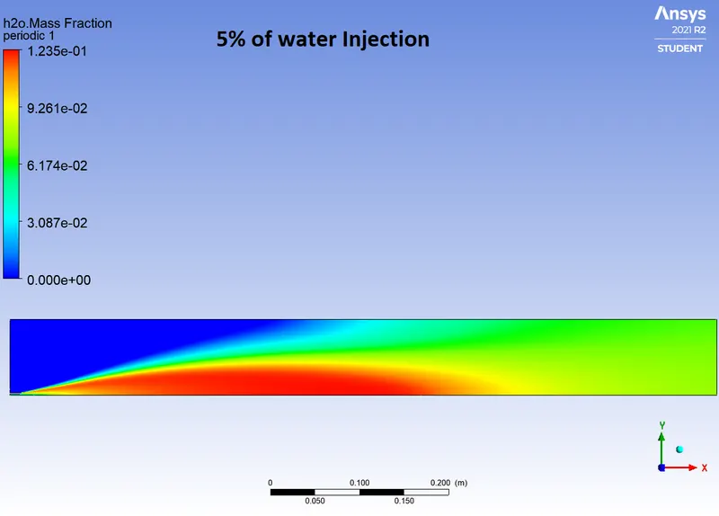
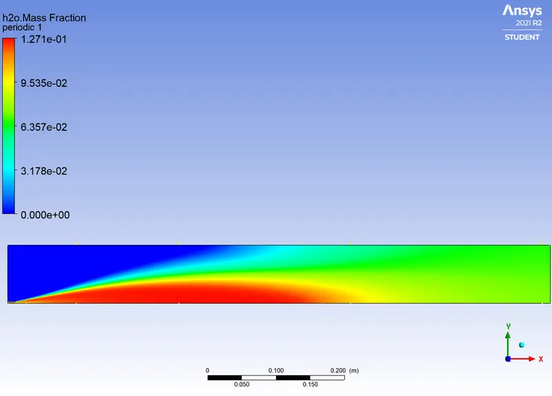
- For second phase of the calculation we add the water of mass fractions 5% , 10%, 15% , 20% , 25% and 30% of fuel for each cases by using parametric study which is enabled in the boundary conditionsof fuel inlet-> species
- In the report definition output parametres is enabled for Temperature at outlet ,Mass fractions of Soot and Nox at outlet inorder to observe the changes
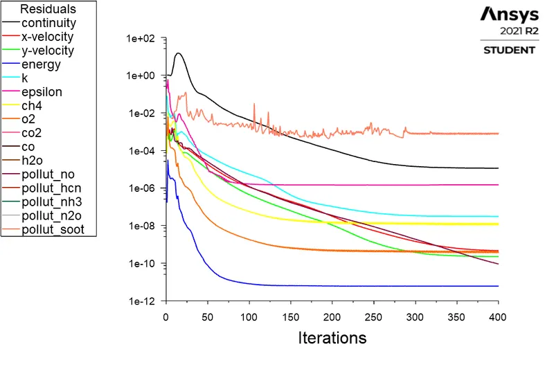
- A hybrid Initialisation with 400 iteration is setup
Outputs
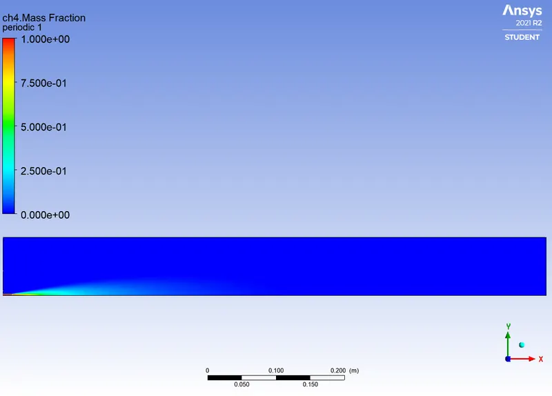
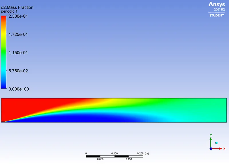
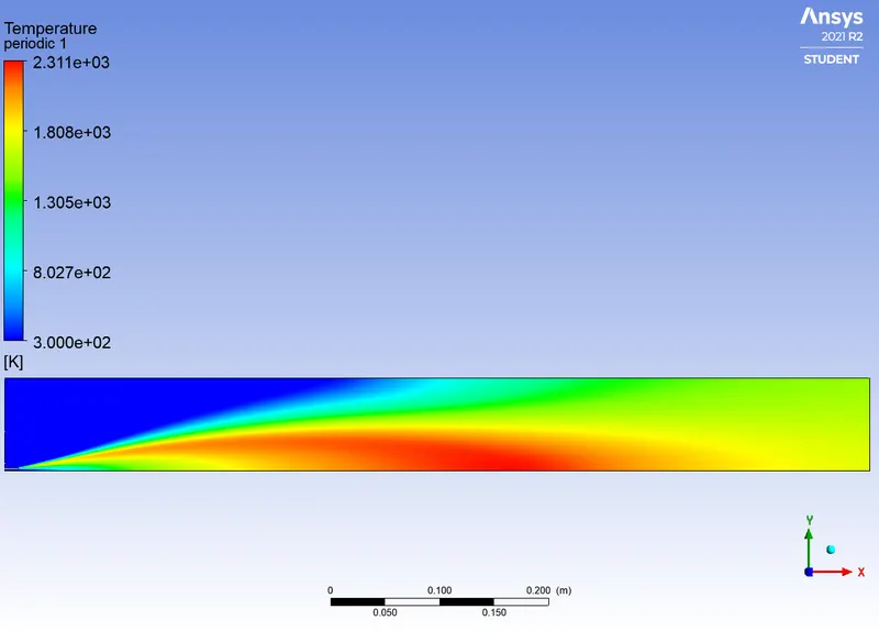
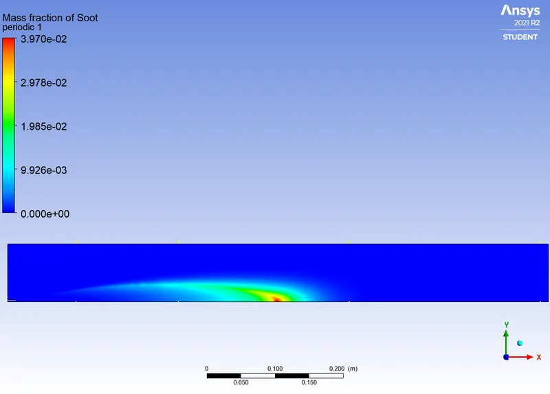
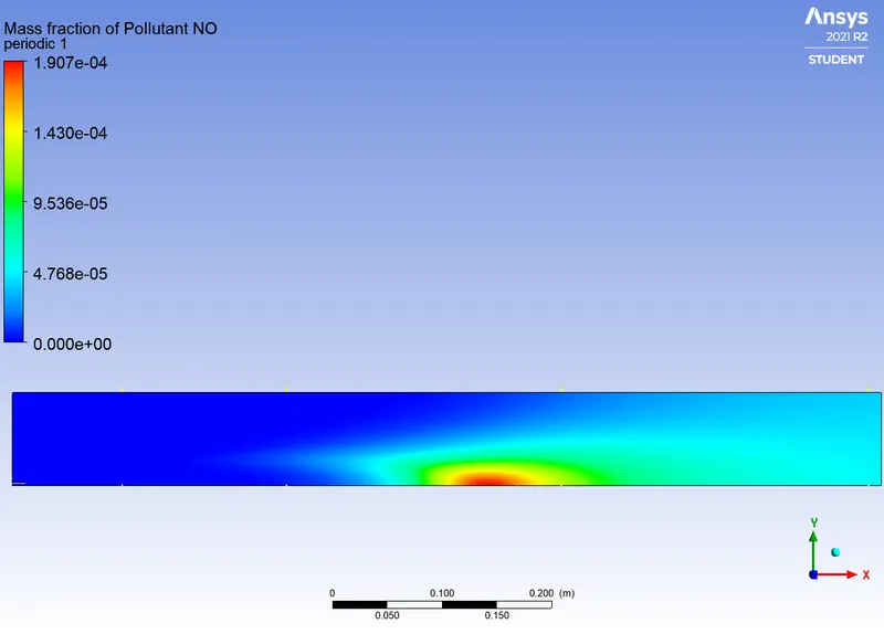
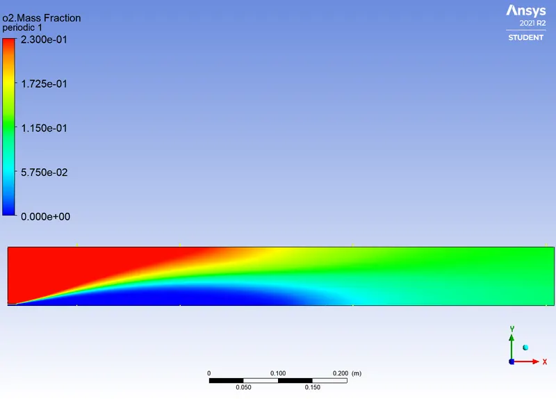
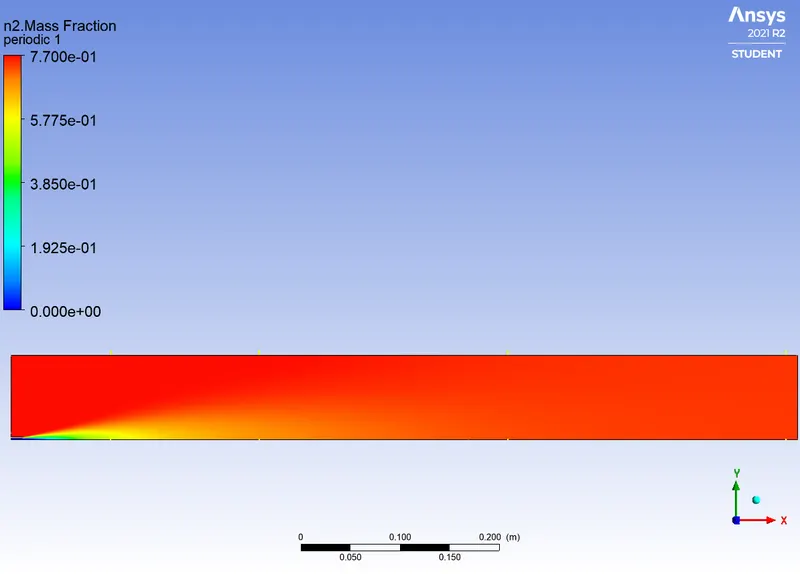
Part 1 - Baseline Simulation (No water injection with fuel)
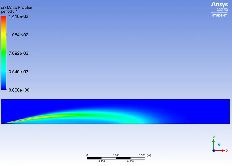
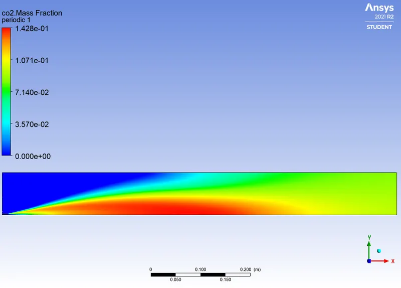
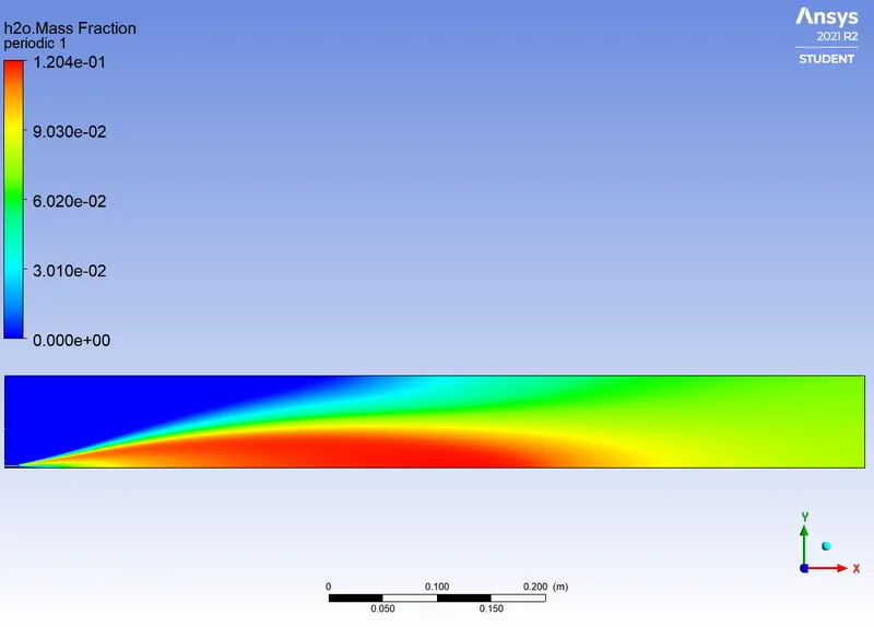
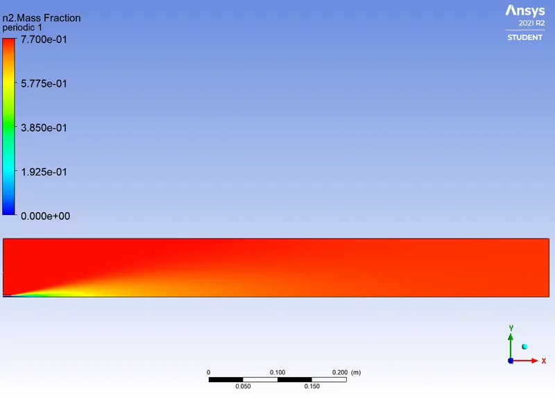
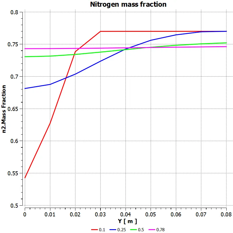
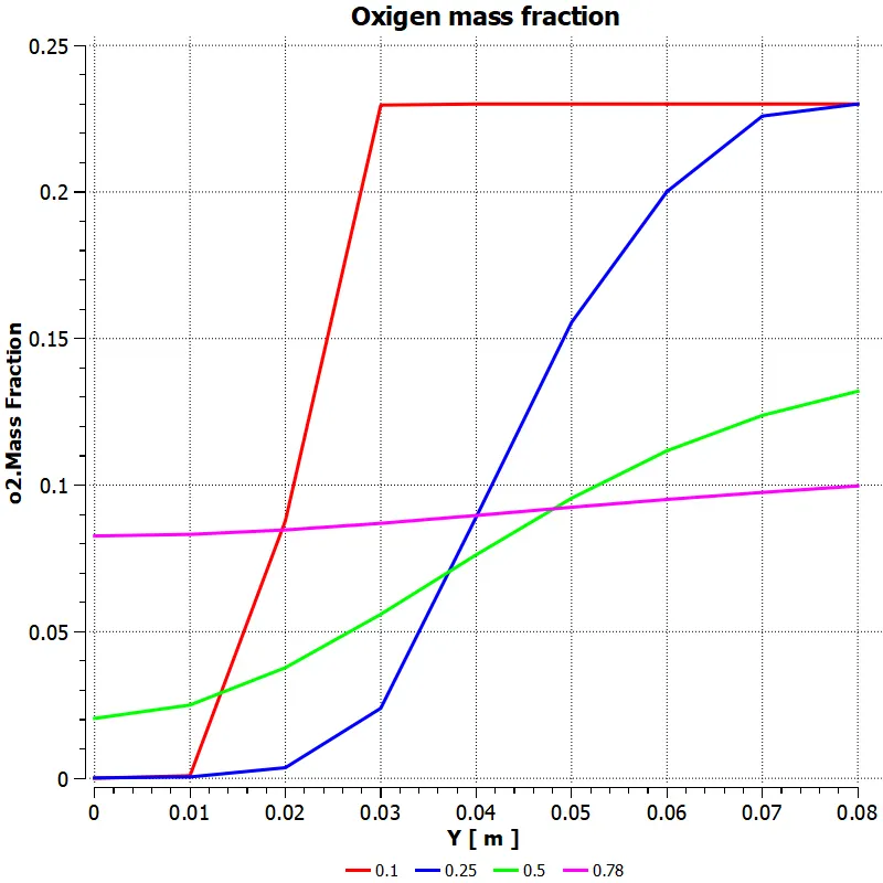
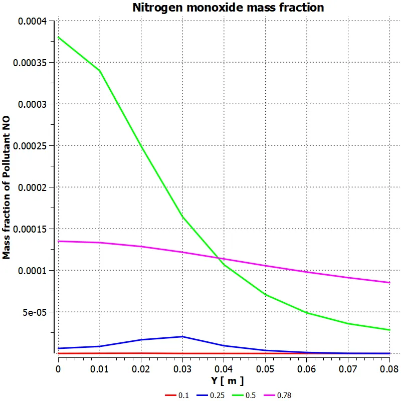
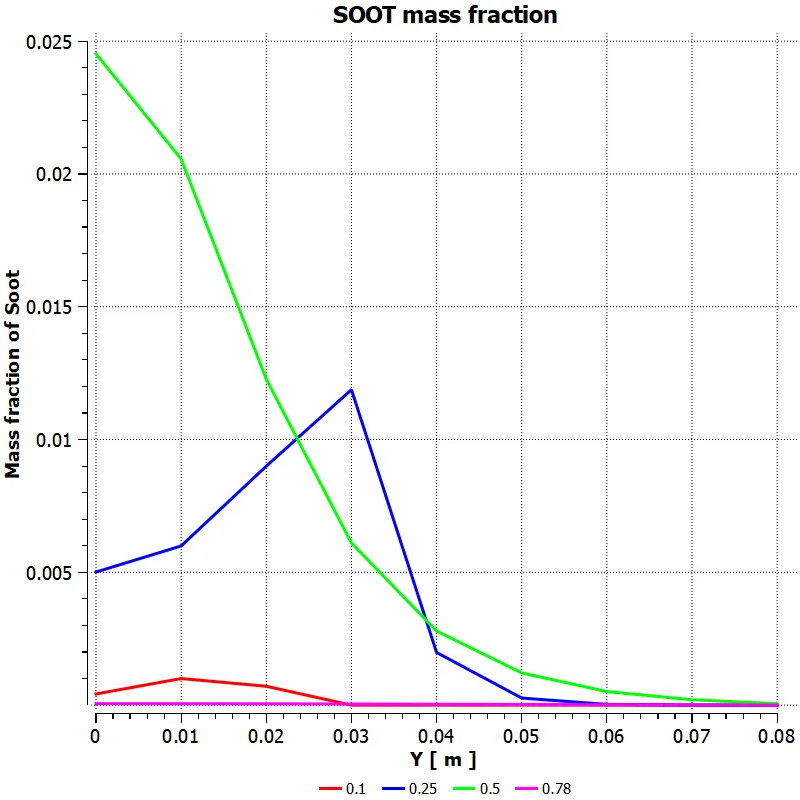
Part 2-
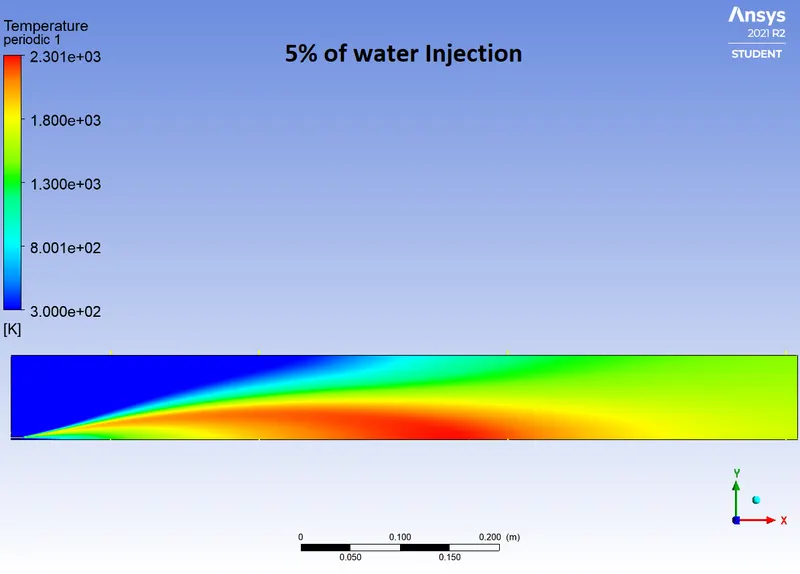
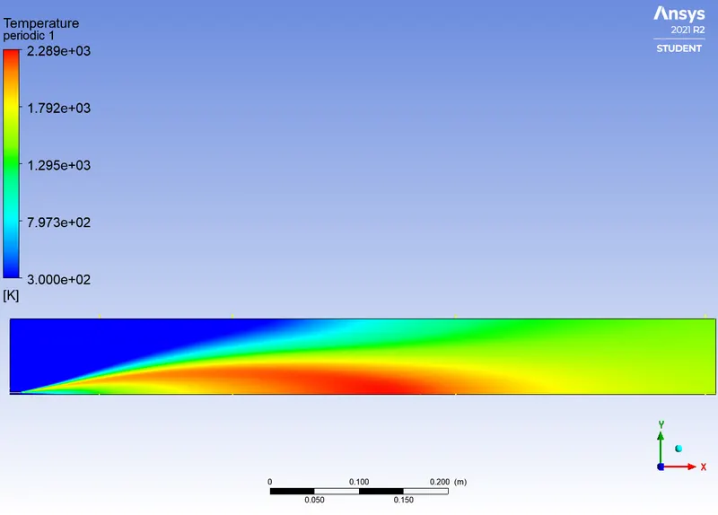
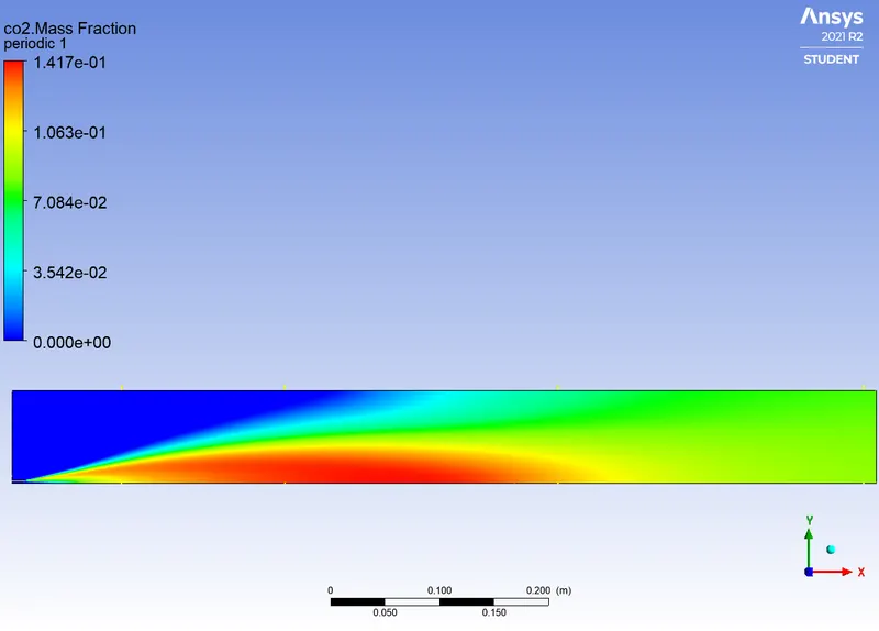
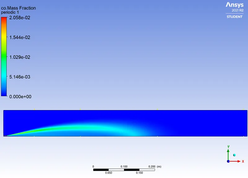
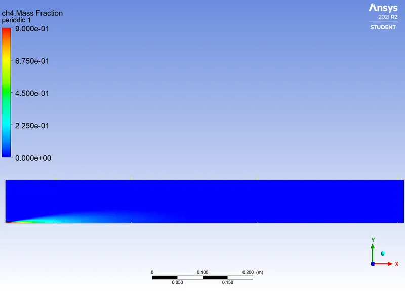
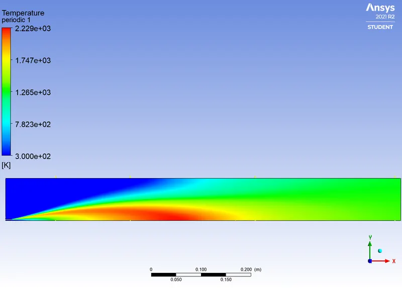
Temperature Contours of Each cases
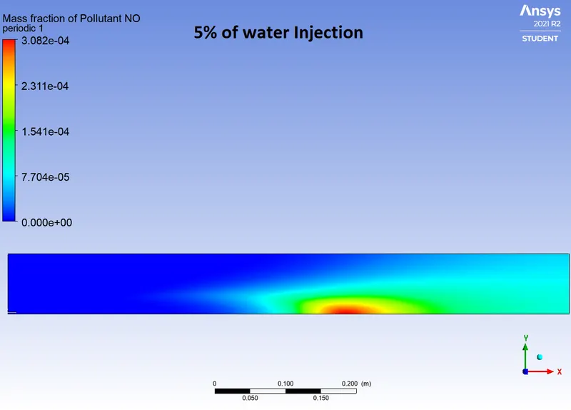
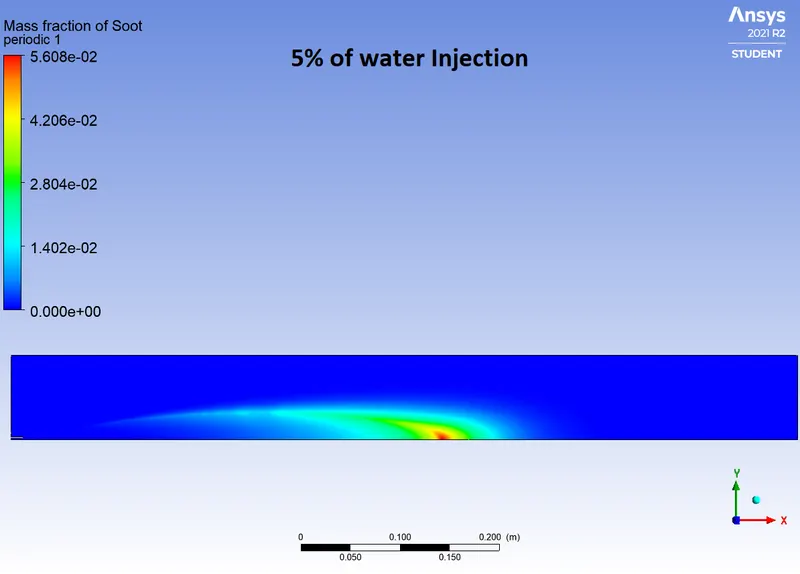
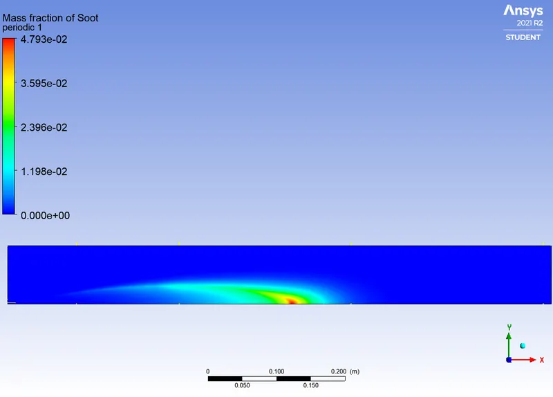
case-1 (5% of water injection)
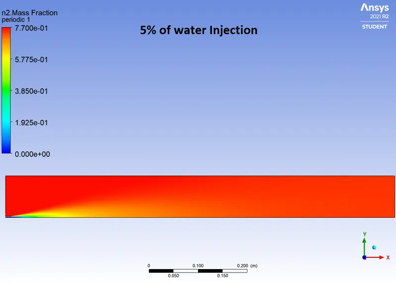
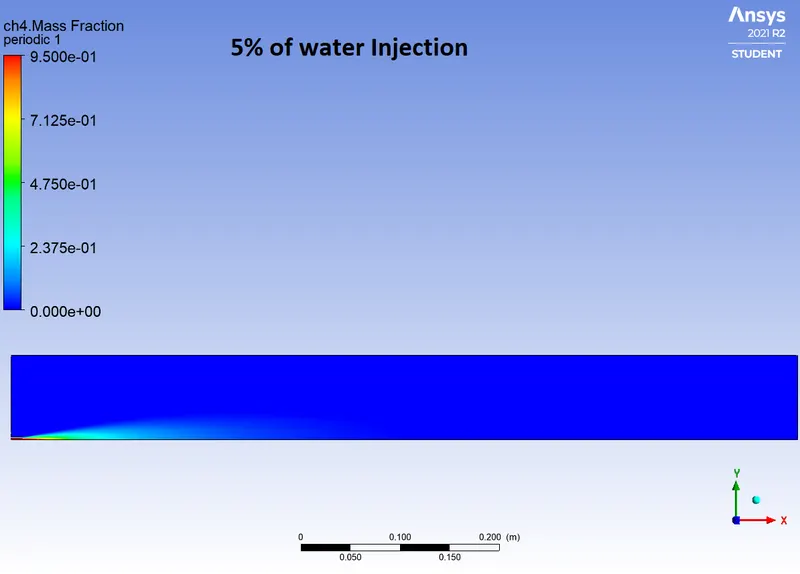
Case 2 - Water Injection 10%
Case 3 - Water Injection 15%
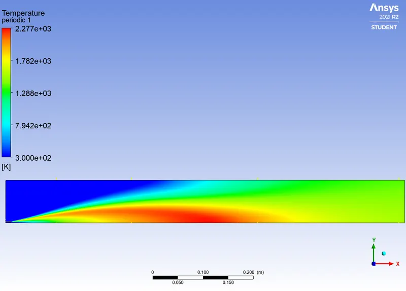
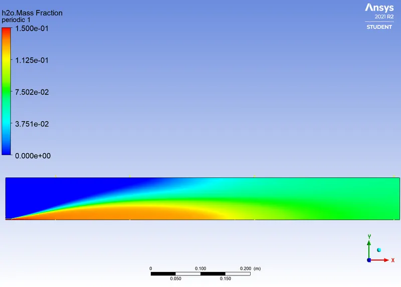
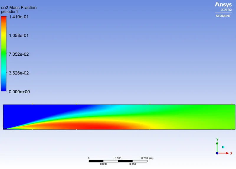
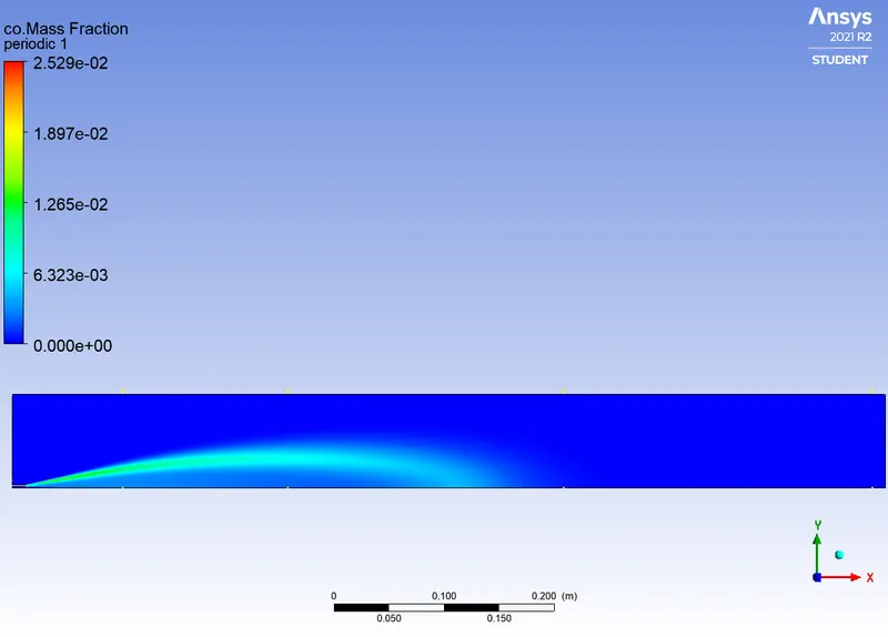
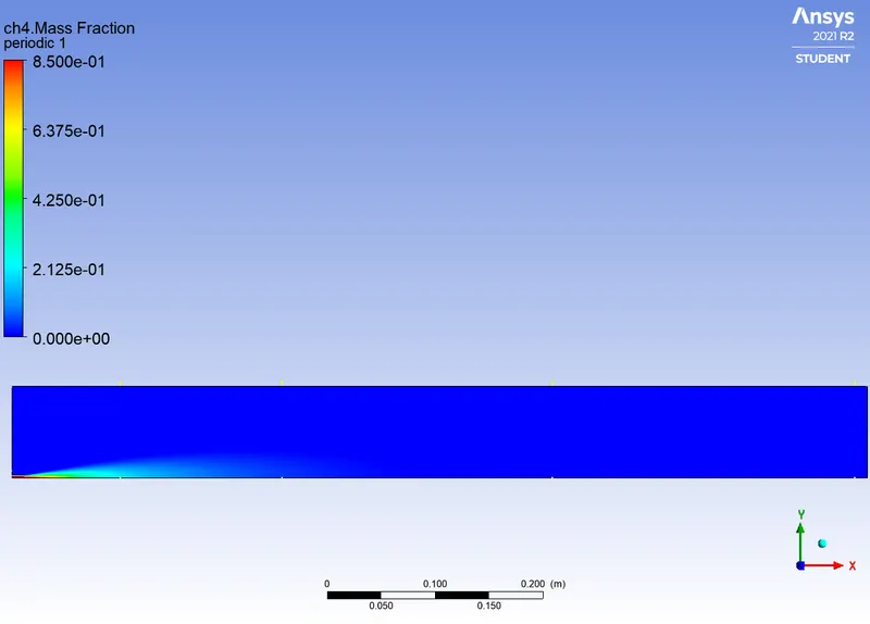
Case 4 - Water Injection 20%
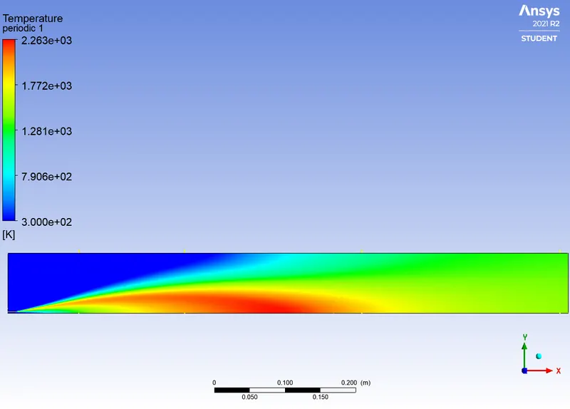
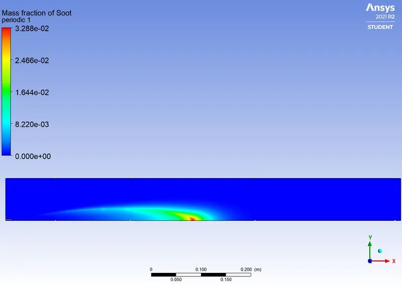
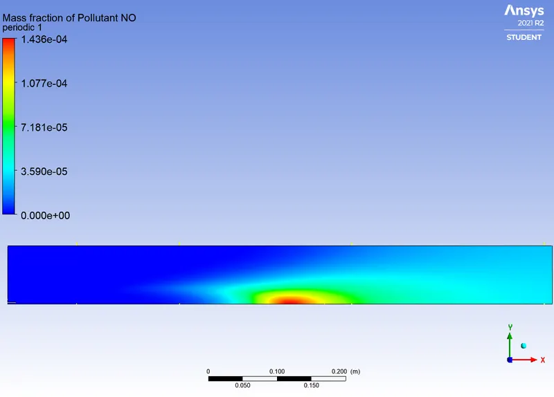
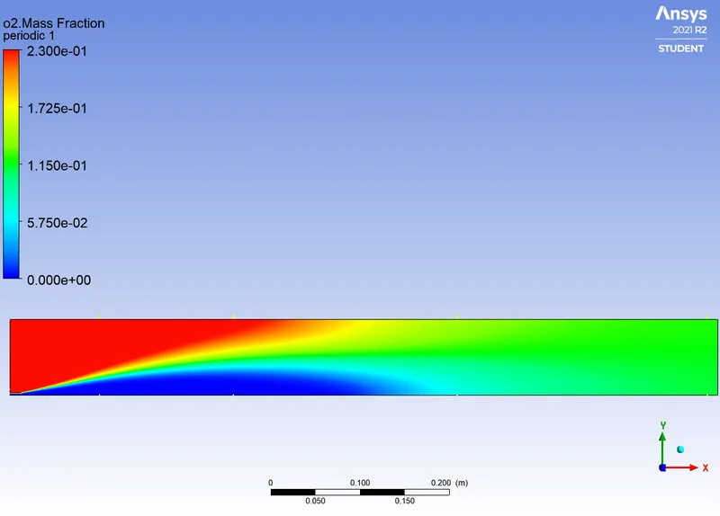
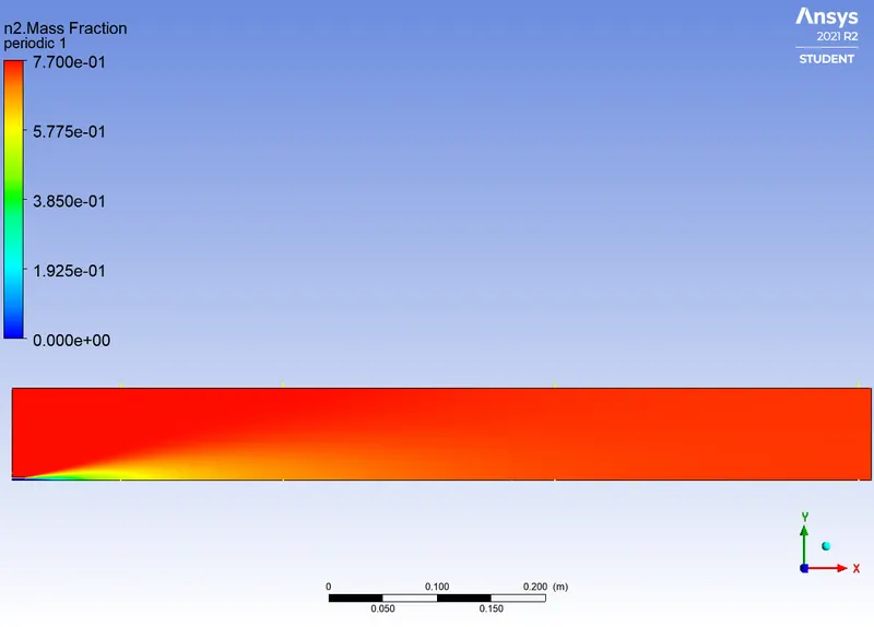
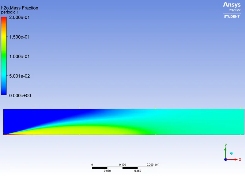
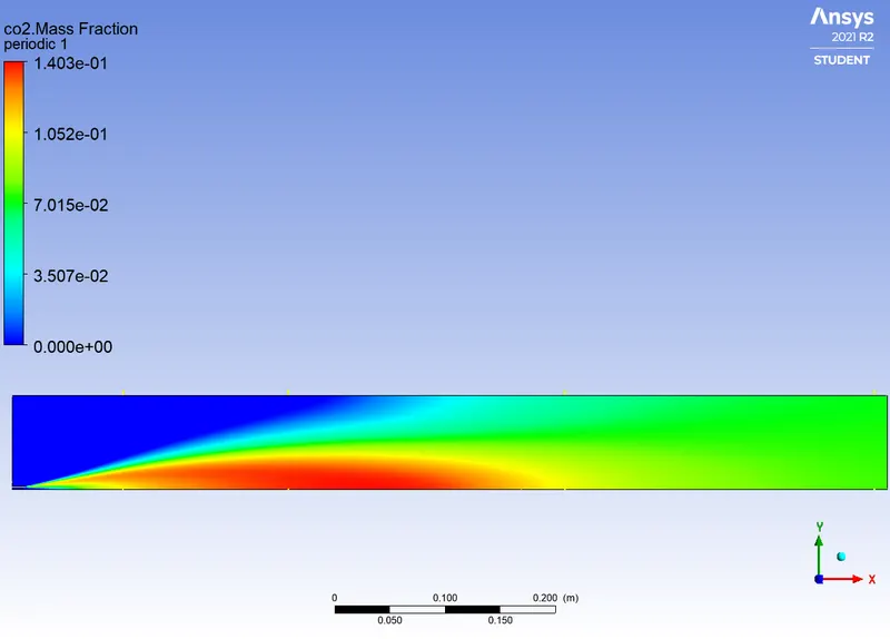
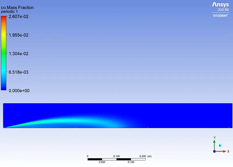
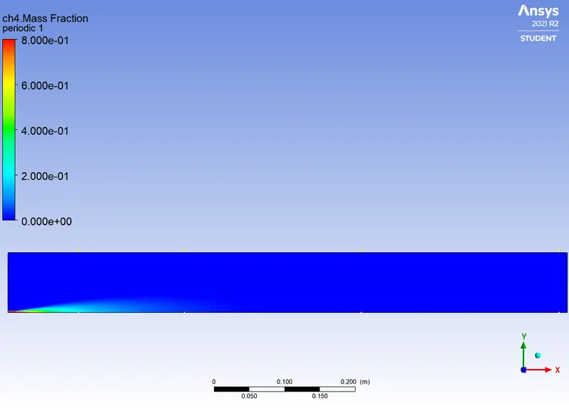
Case 5 - Water Injection 25%
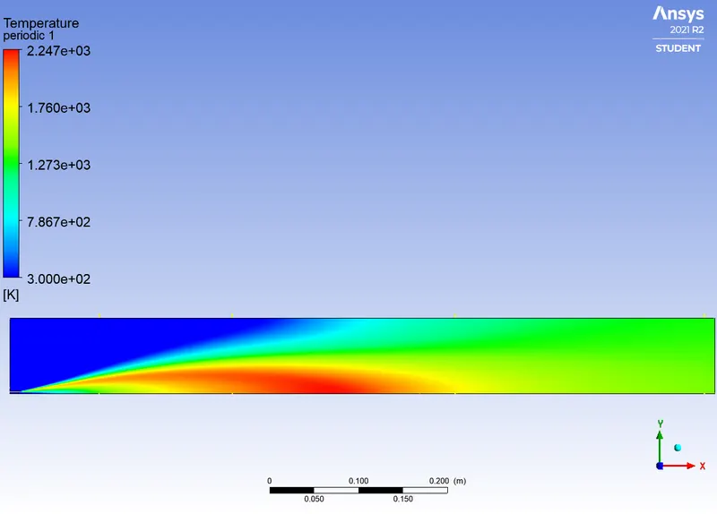
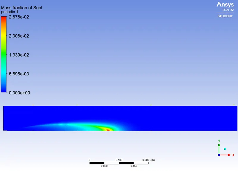
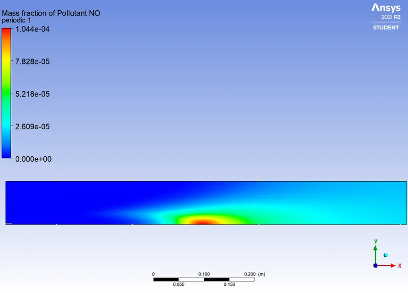
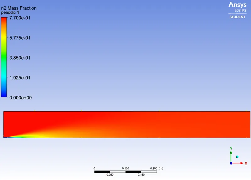
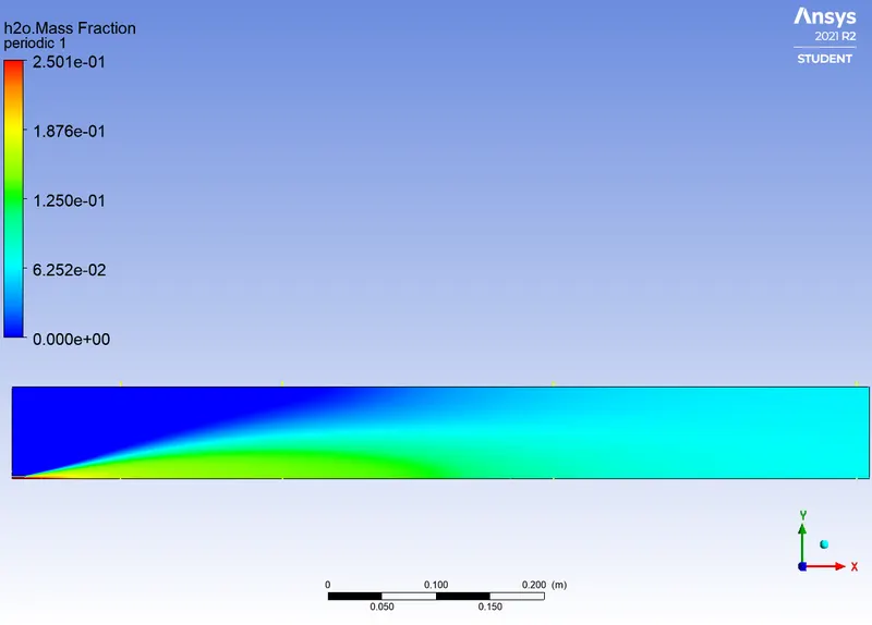
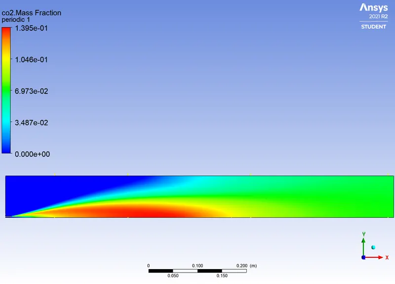
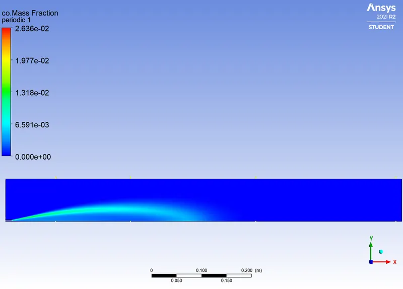
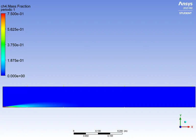
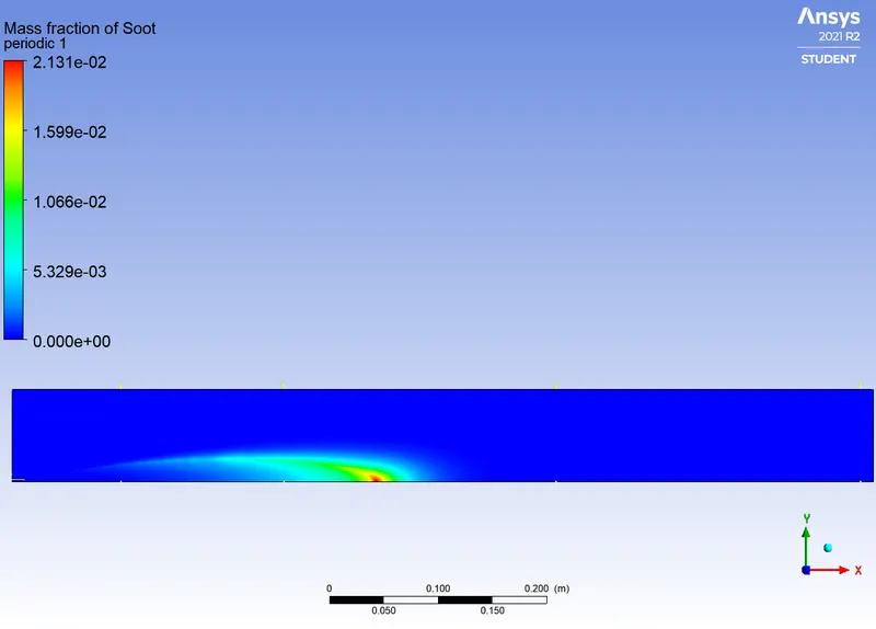
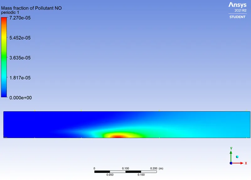
Case 6 - Water Injection 30%
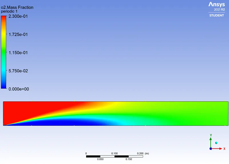
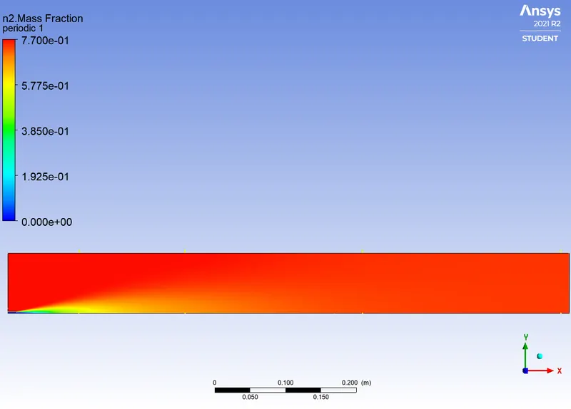
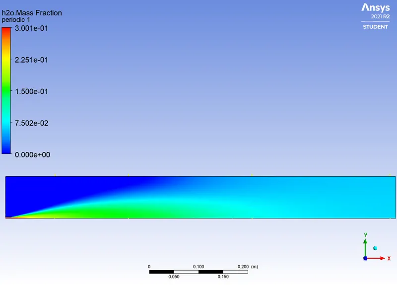
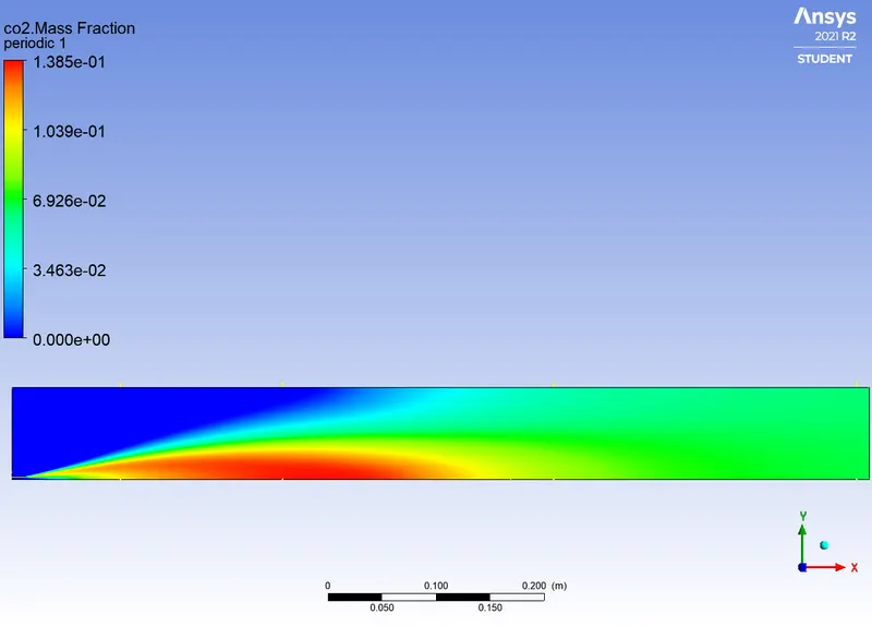
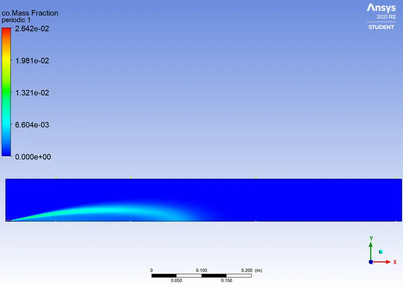
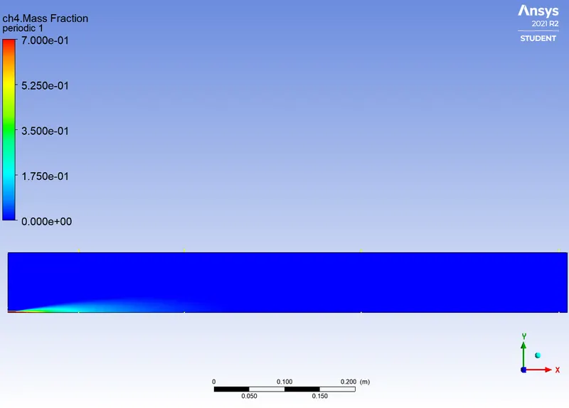
Plots
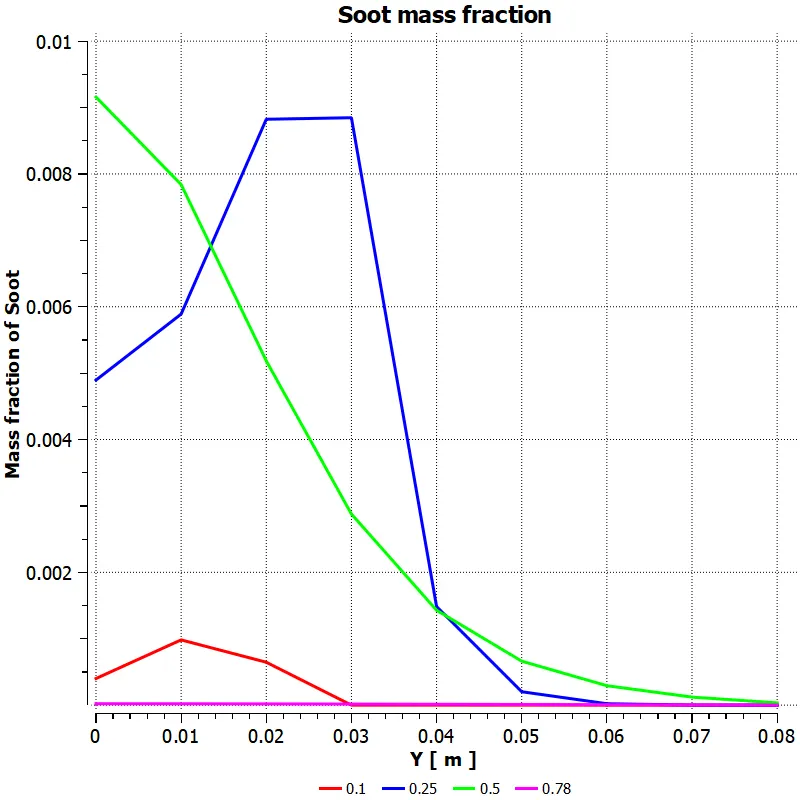
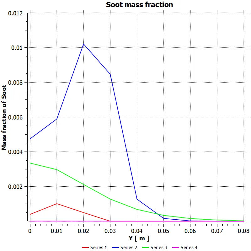
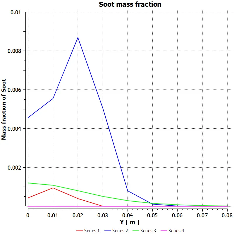
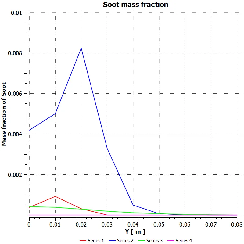
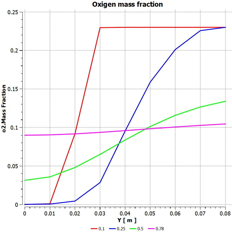
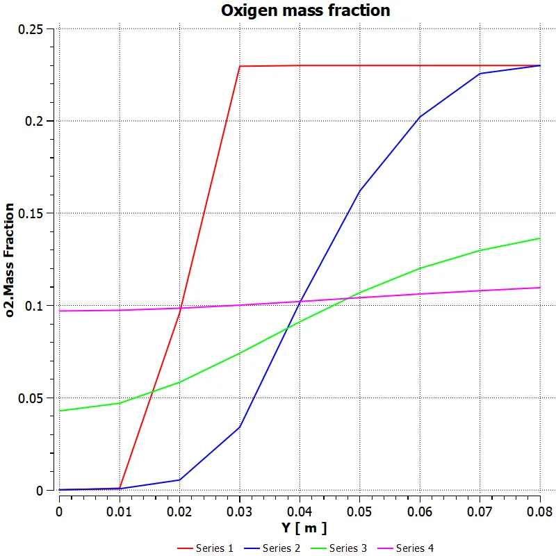
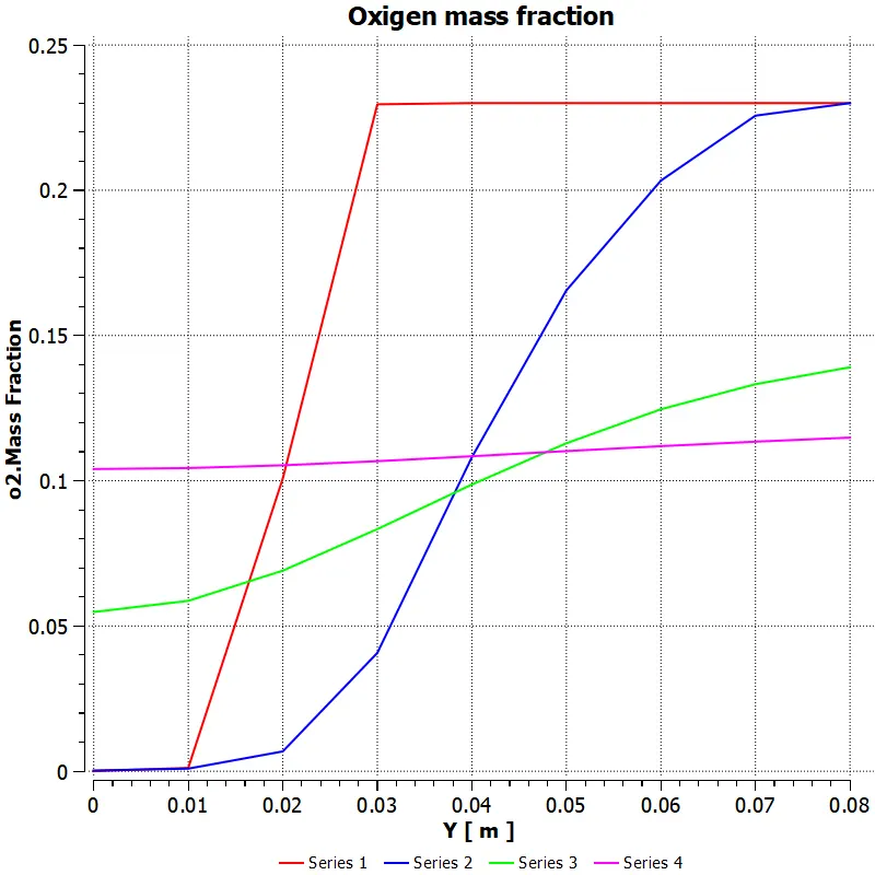
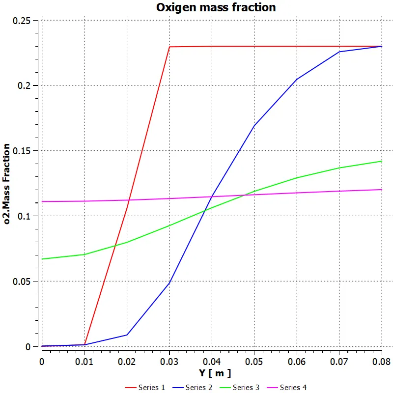
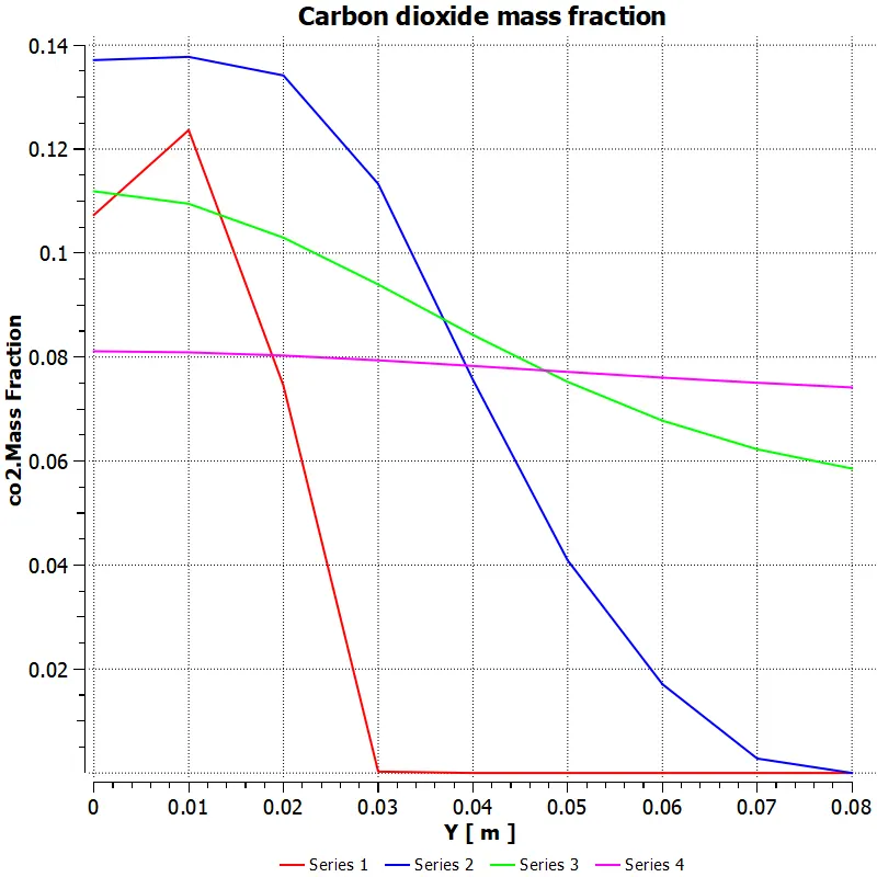
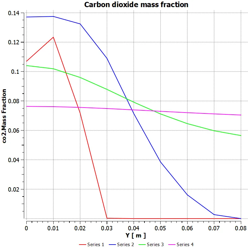
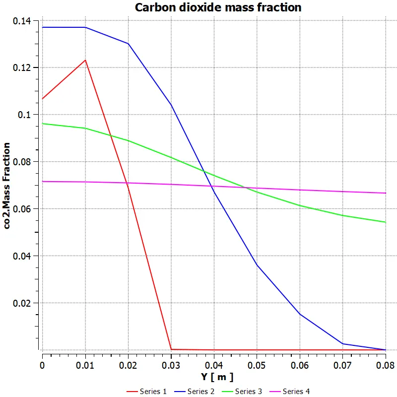
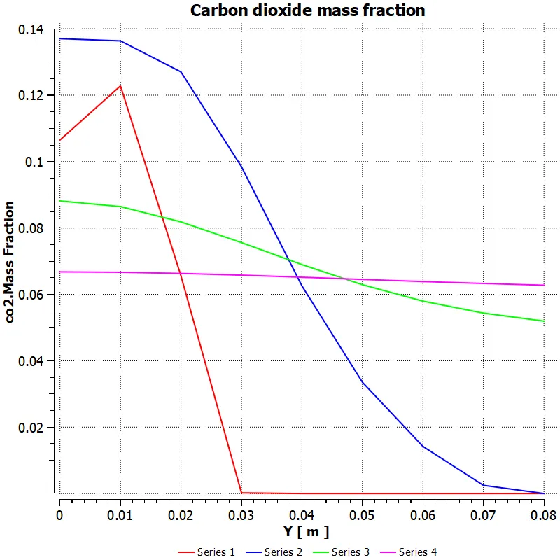
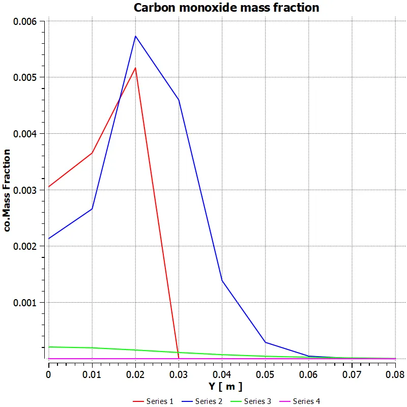
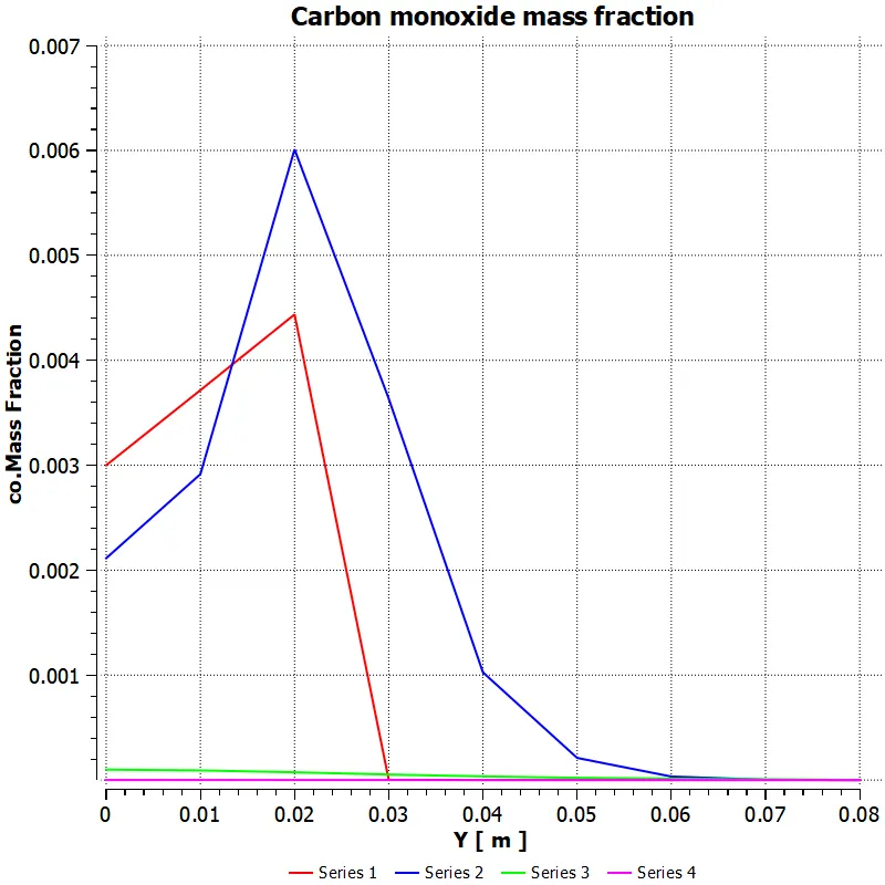
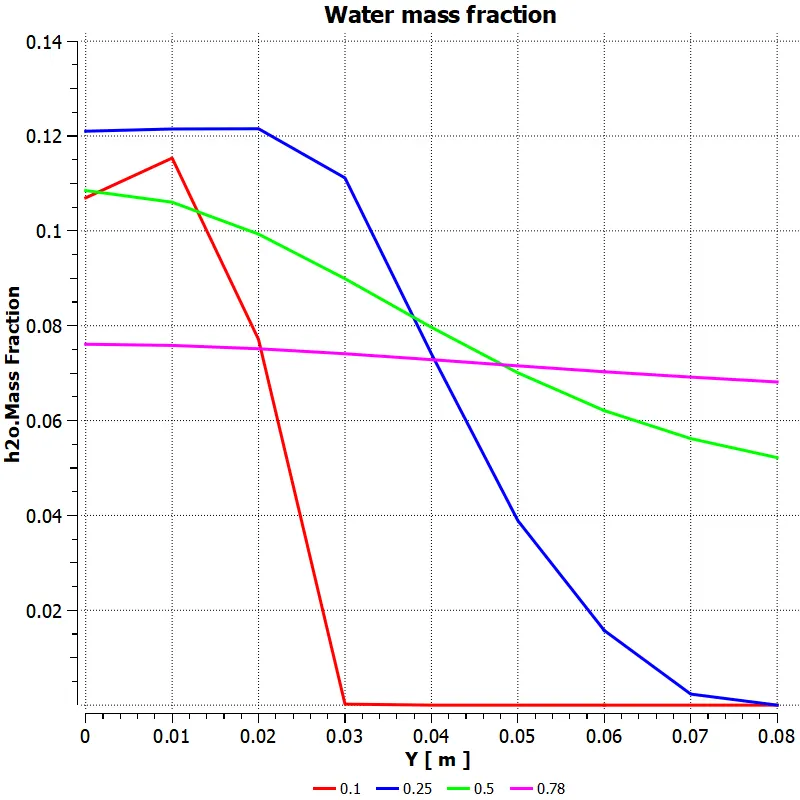
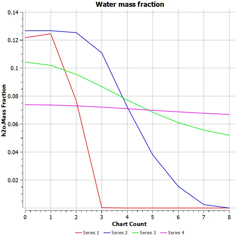
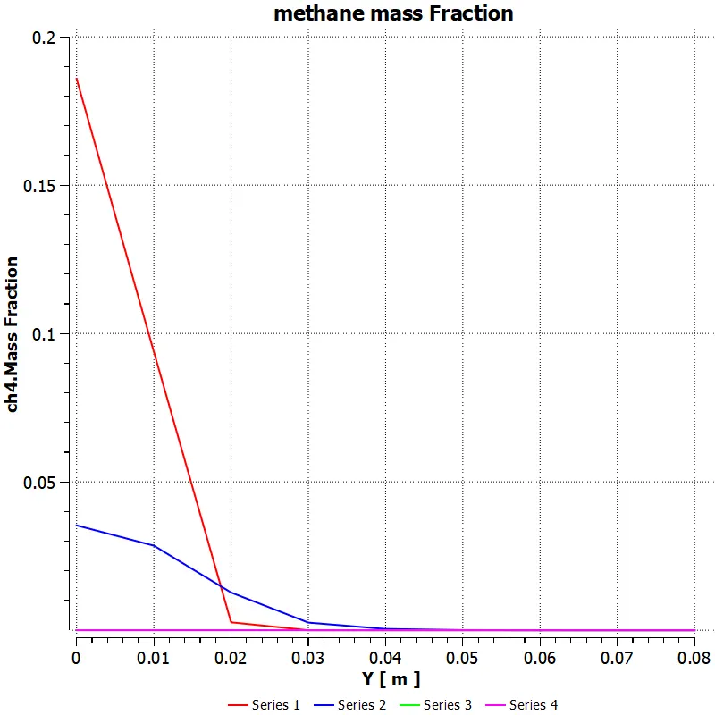
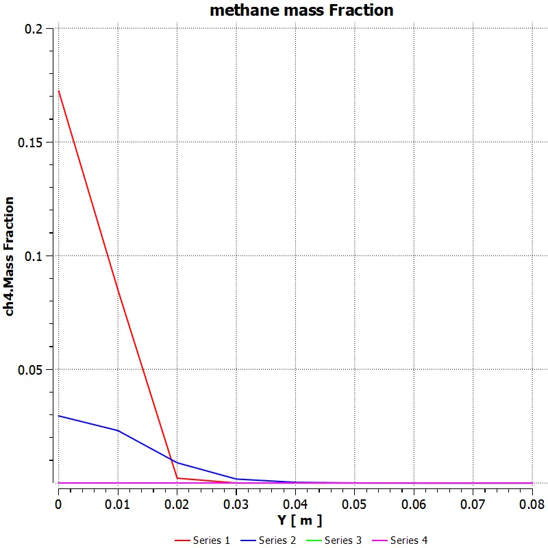
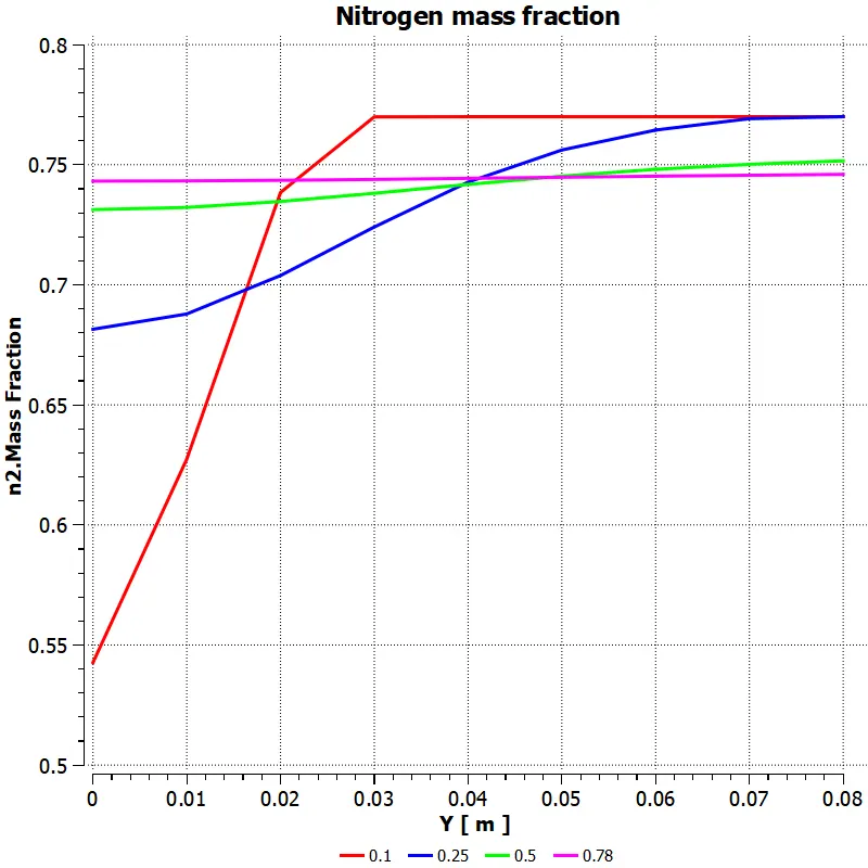
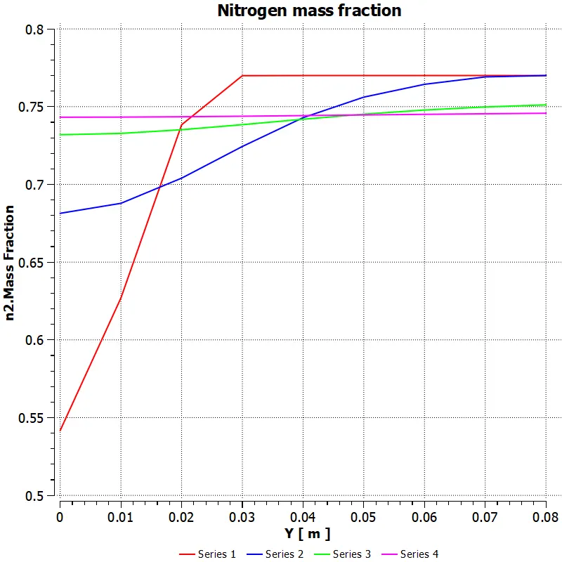
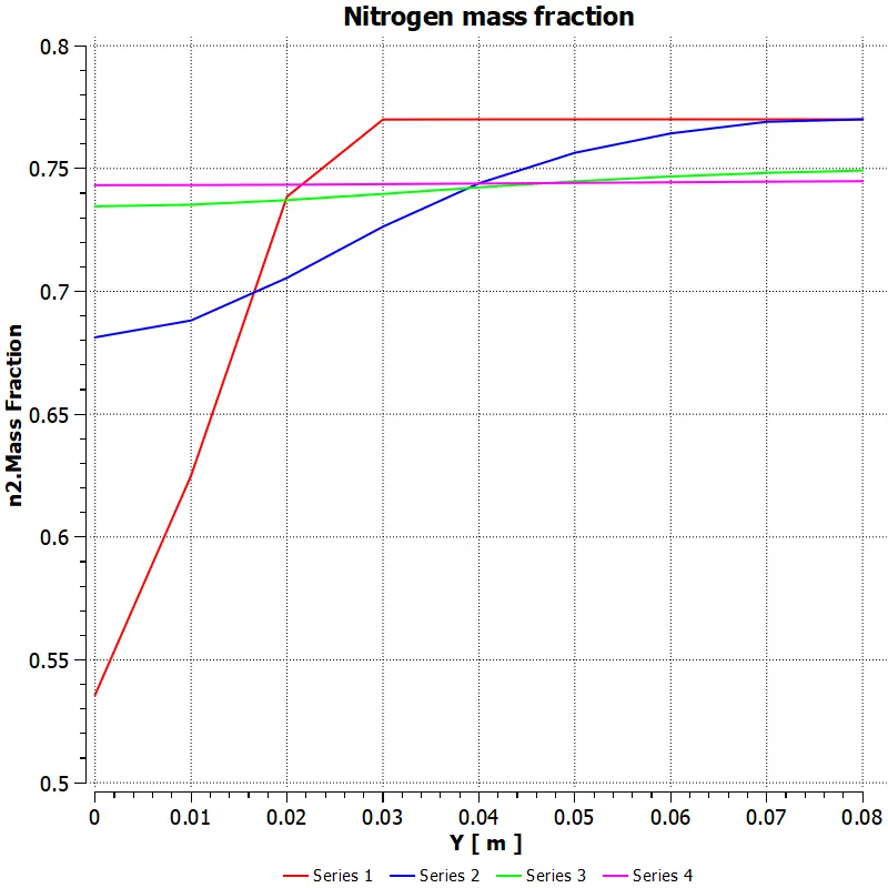
- In the post processor I have created four lines as shown in picture below. Four of them are placed in a way to capture the variation of specific parametres
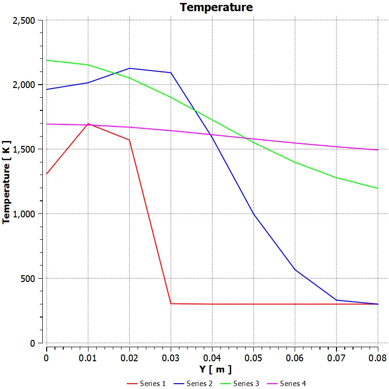
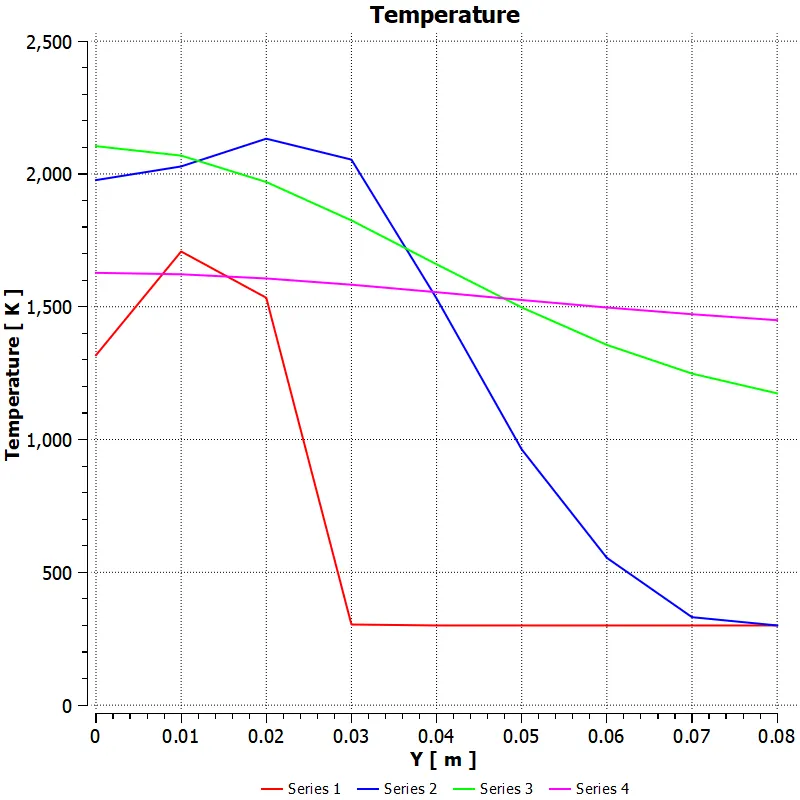
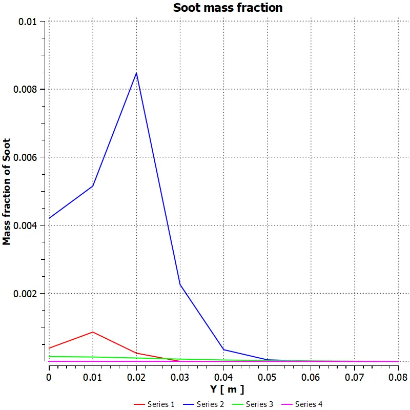
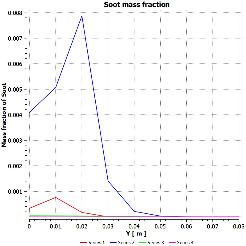
- Series 1 , Series 2, Series 3 and Series 4 represents the Line 1,Line 2,Line 3 and Line 4 respectively
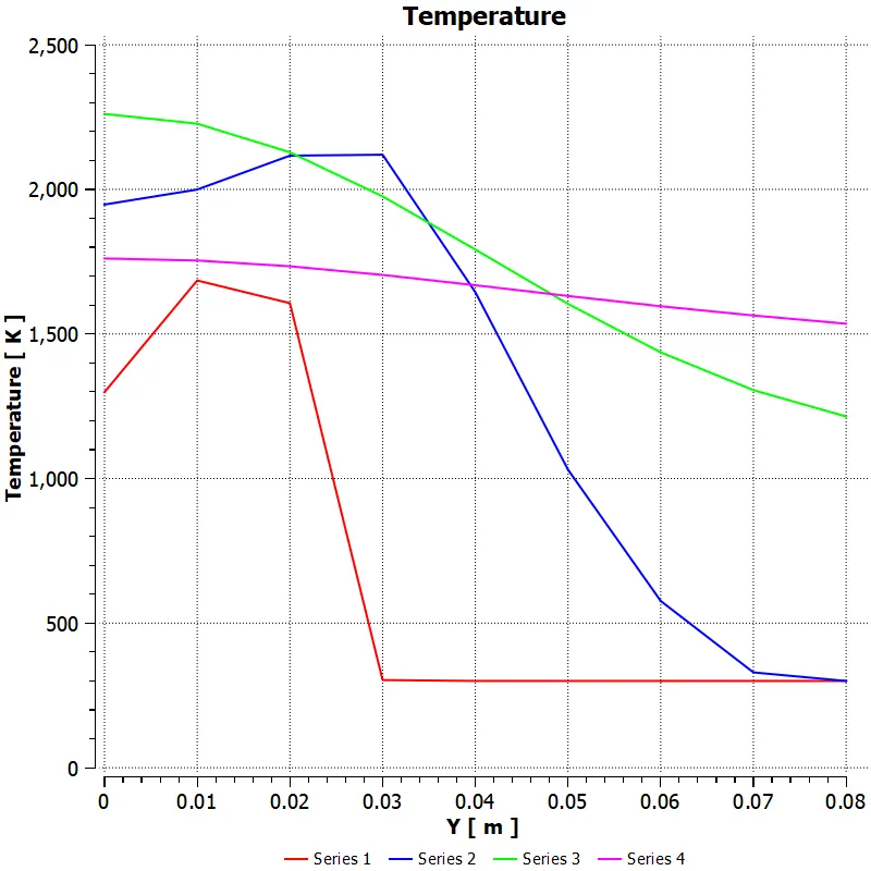
Comparison of Temperature plots of each cases
- For Case 1
- For case 2
- For case 3
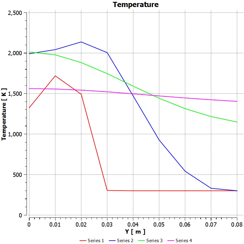
- For case 4
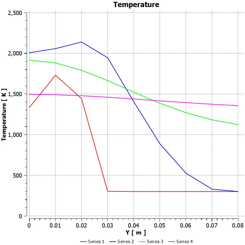
- For case 5
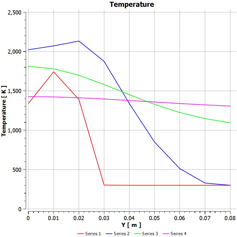
- For case 6
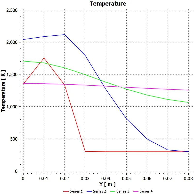
Observations
- As the percentage of water is increased the temperature at the outlet is getting lower
Comparison of soot plots of each cases
- Case 1
- Case 2
- Case 3
- Case 4
- Case 5
- Case 6
Observations
- Soot is formed more where the Line 2 lies and as expected the Soot is gettin reduced by injecting water, greater the percentage of injection lower the Pollutant
Comparison of NO plots of each cases
- Case 1
- Case 2
- Case 3
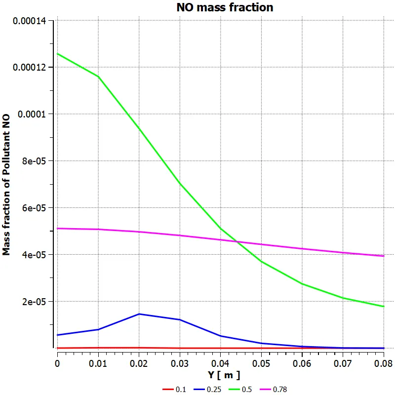
- Case 4
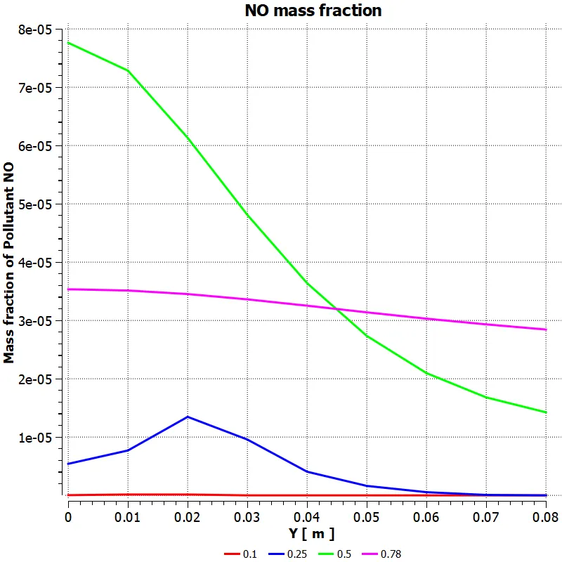
- Case 5
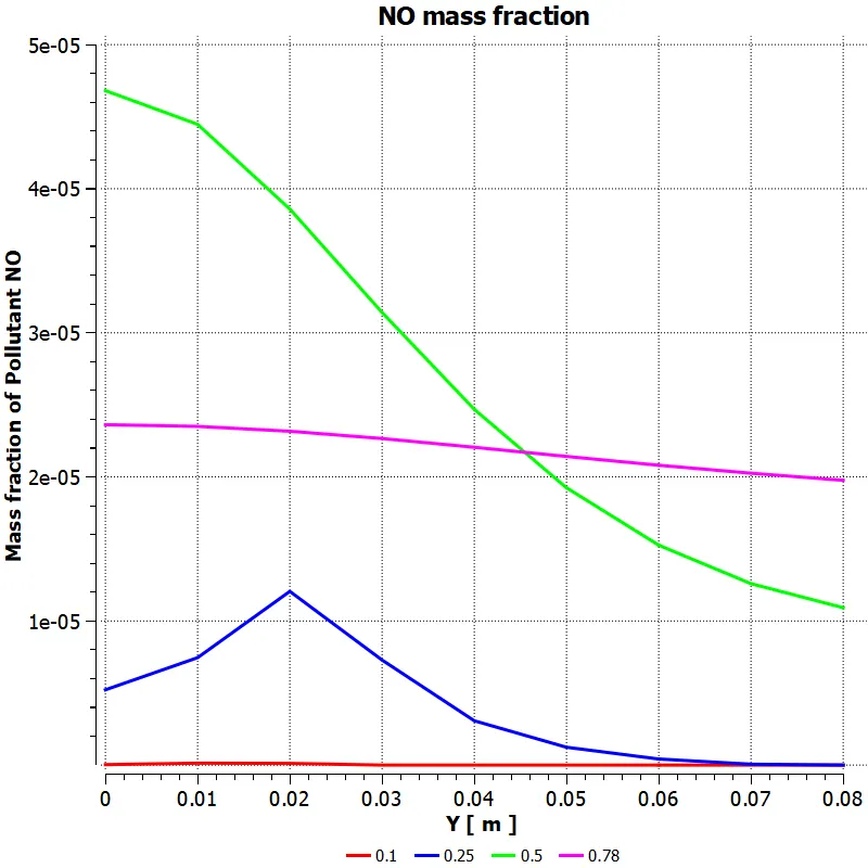
- Case 6
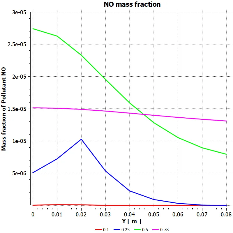
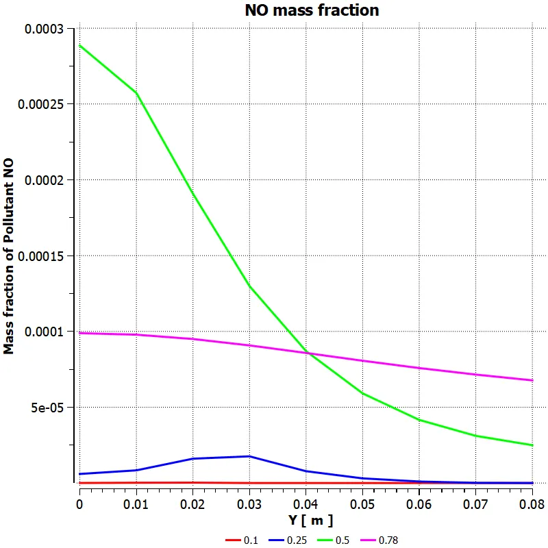
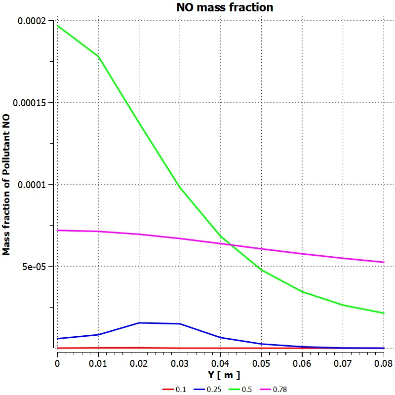
- Nitrogen monoxide is produced more where the line 3 is placed
- Also the production of the pollutant is getting lower on each cases (due to more injection of water)
Comparison of Oxigen plots of each cases
- Case 1
- Case 2
- Case 3
- Case 4
- Case 5
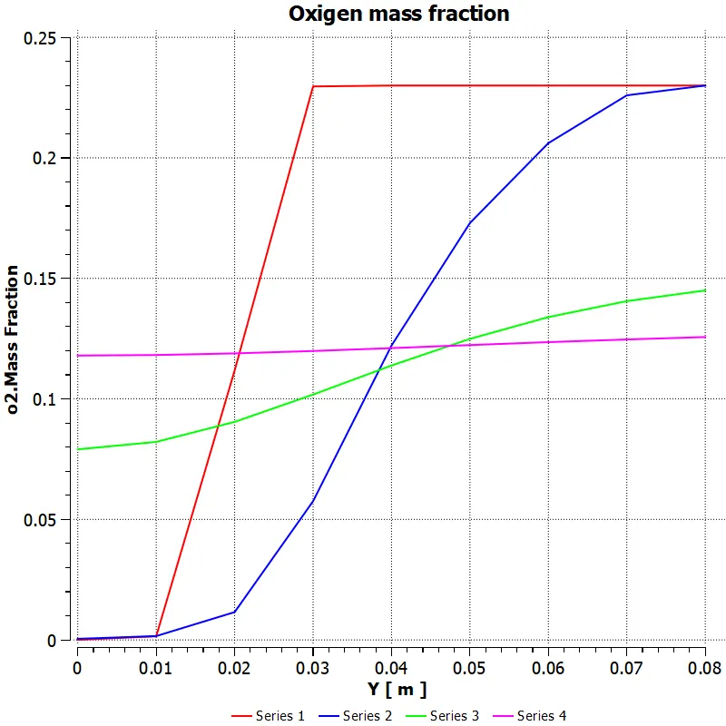
- Case 6
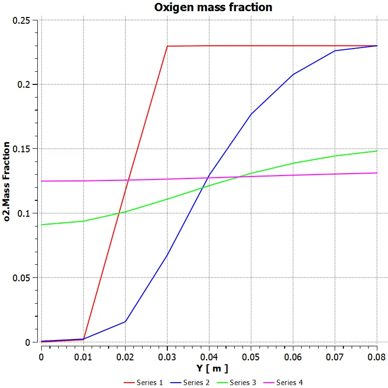
Observations
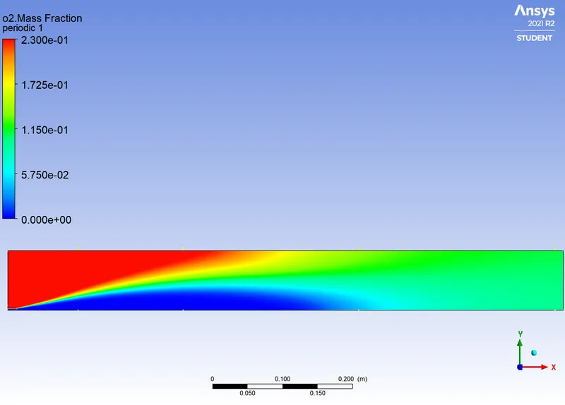
- Since Line 1 is near to the inlet the oxygen is present more there
- On first 2 lines there doesnt seem to have changes but when we observe Line 3 and Line 4 variations we can conclude that the Oxigen availibility is getting more by the injection of water
Comparison of Carbon dioxide plots of each cases
- Case 1
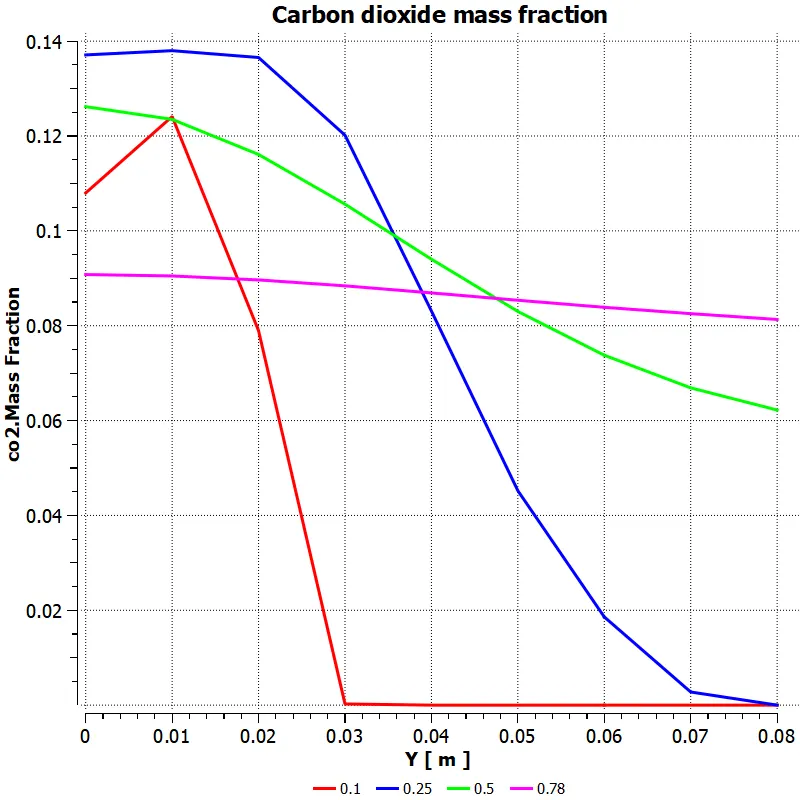
- Case 2
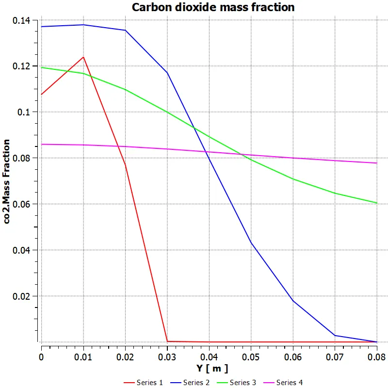
- Case 3
- Case 4
- Case 5
- Case 6
Observations
- CO2 seems to have formed more where line 2 lies and there is no much of a change (for line 2 curve) in each cases
- Also the CO2 at the outlet is getting lower as injection of water is incresed
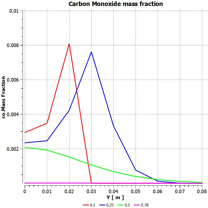
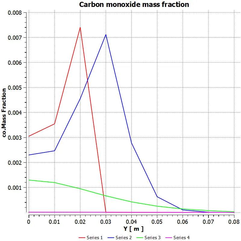
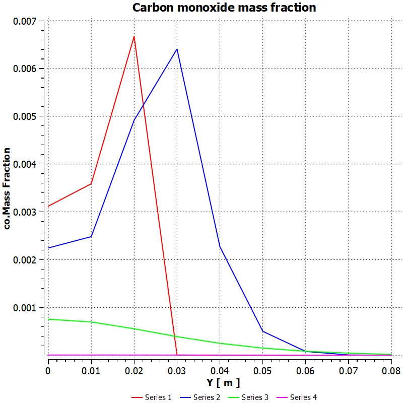
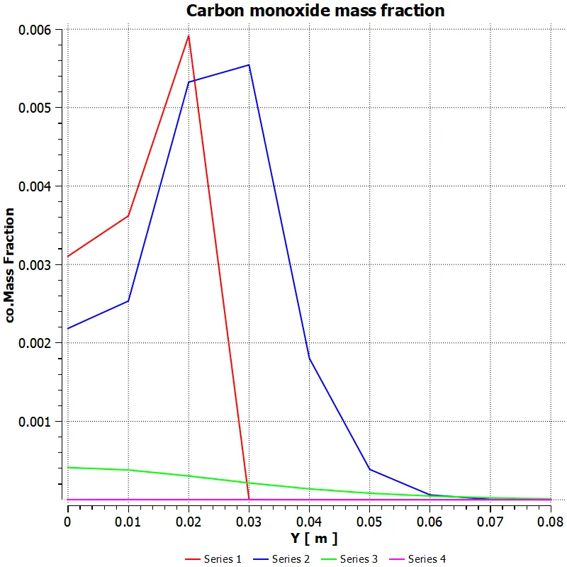
Comparison of Carbon Monoxide plots of each cases
- Case 1
- Case 2
- Case 3
- Case 4
- Case 5
- Case 6
Observations
- Carbon monoxide is also present more at the regions of line 1 and line 2 and quantity of it getting produced is lowered by the introduction of water
Water plots of each cases
- Case 1
- Case 2
- Case 3
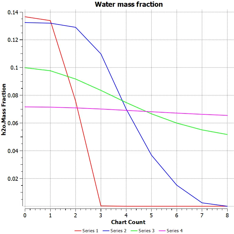
- Case 4
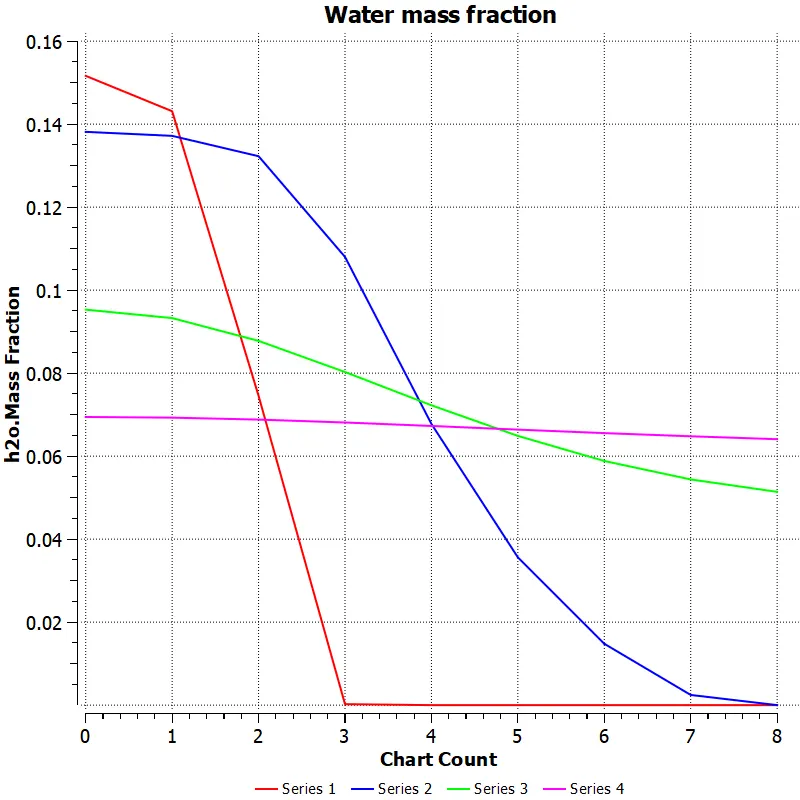
- Case 5
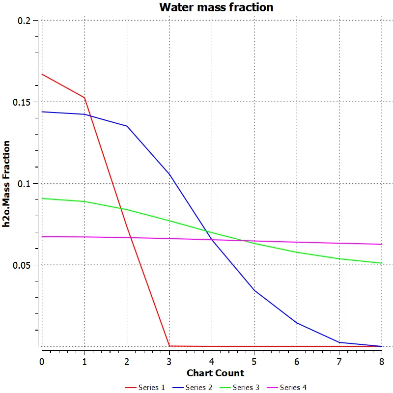
- Case 6
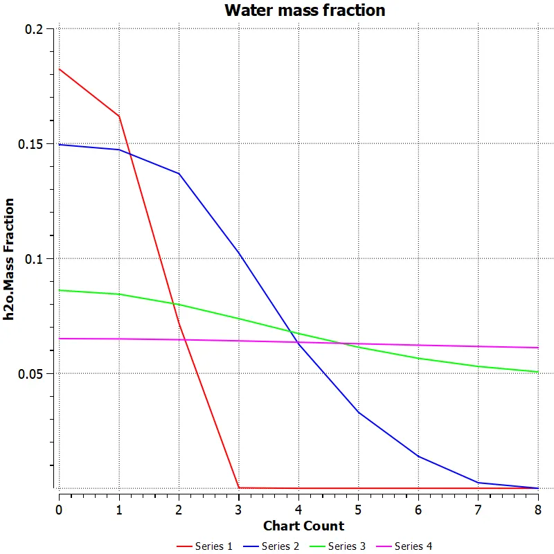
Methane mass fractions of each cases
- case 1
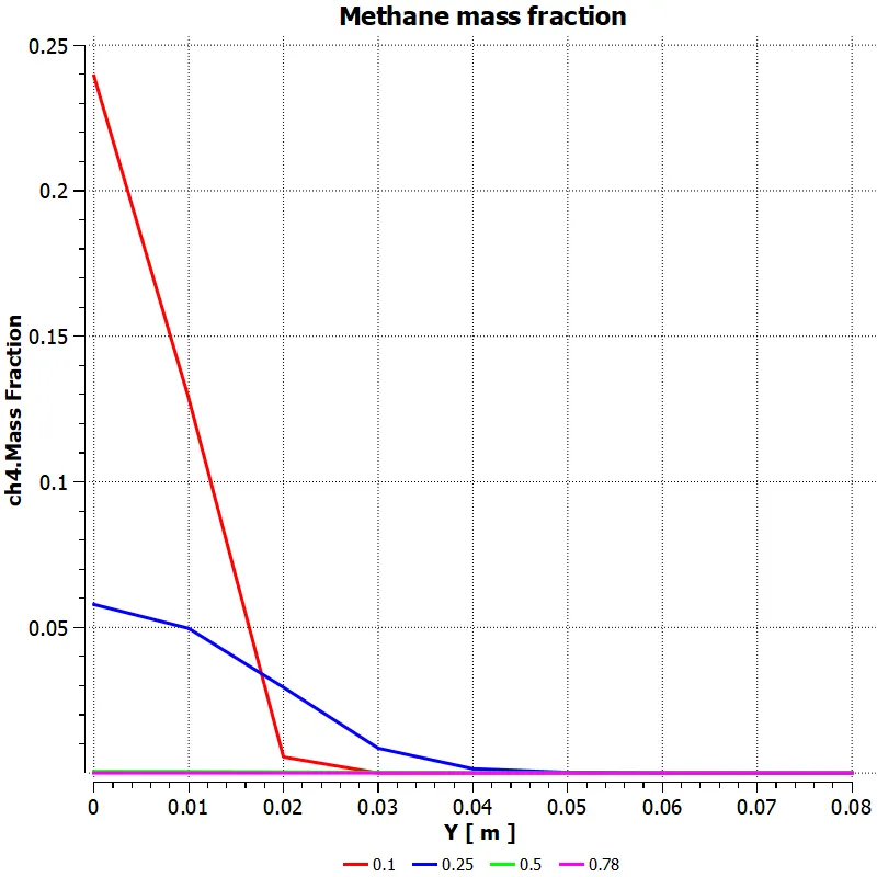
- case 2
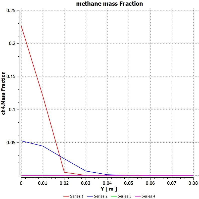
- case 3
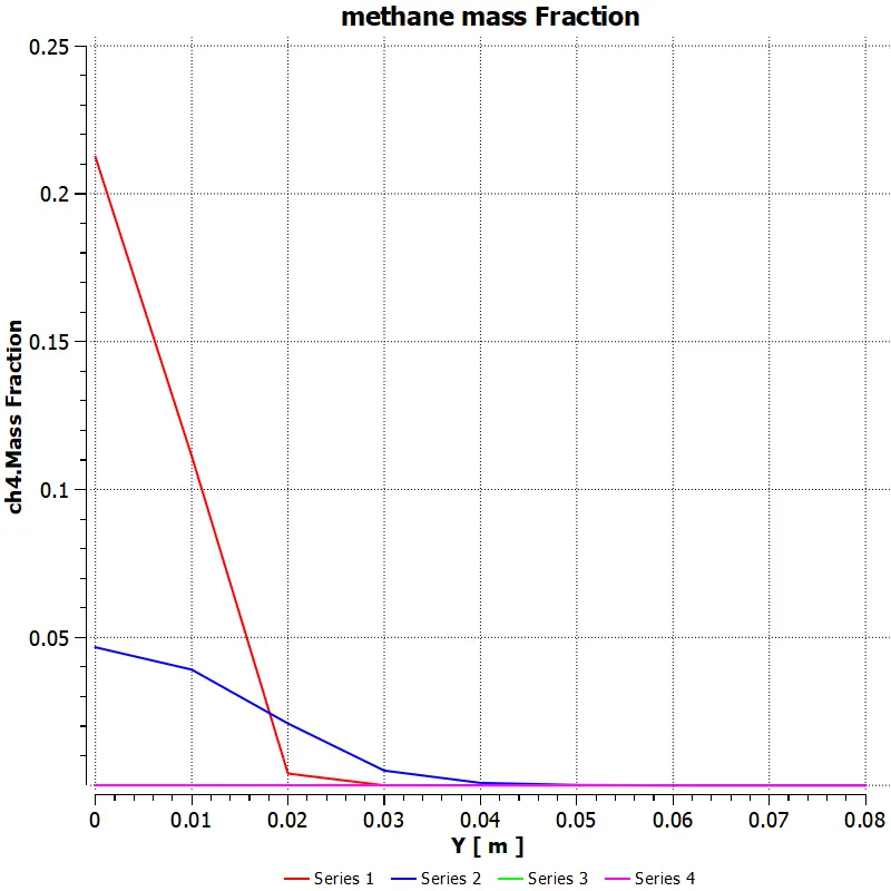
- case 4
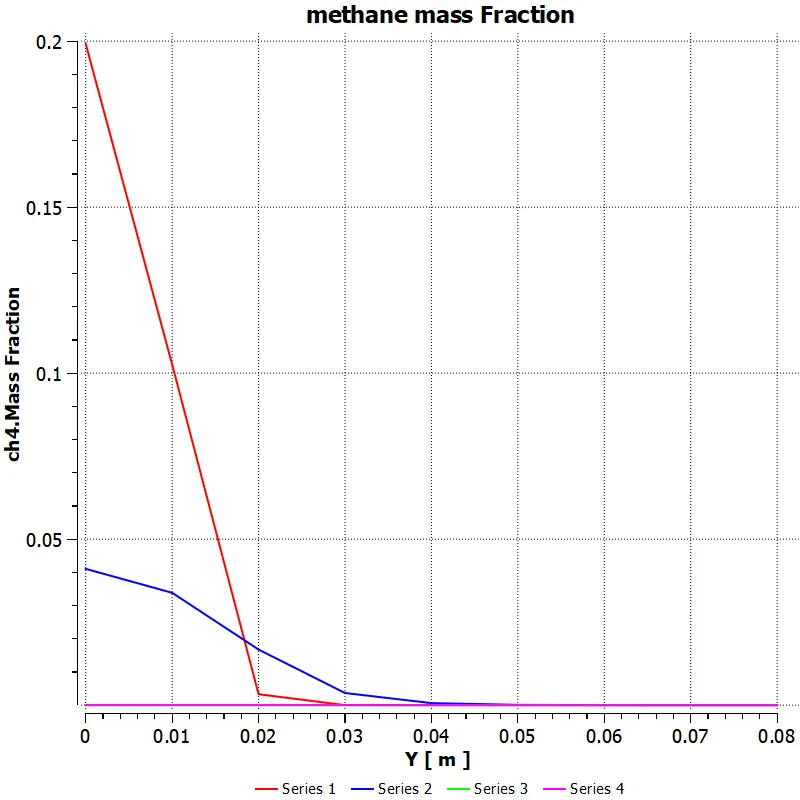
- case 5
- case 6
Nitrogen mass fractions of each cases
- case 1
- case 2
- case 3
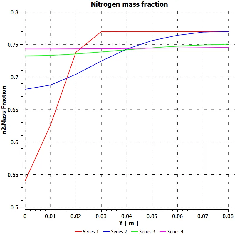
- case 4
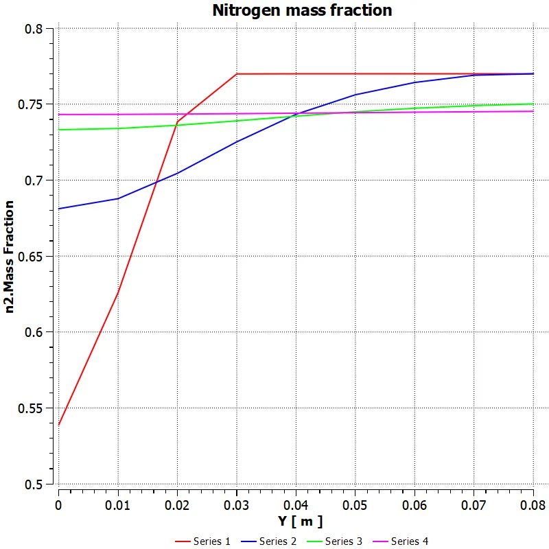
- case 5
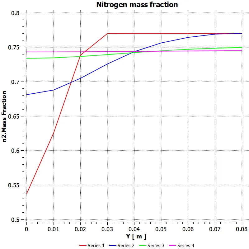
- case 6
Parametric table
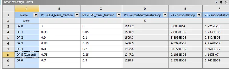
- Through the observstion of the values of pollutants and the temperatures obtained for each simulation we can confirm the fact that injecting water by a 30% is more effective in reducing the pollutants getting formed
- Since I haven't selected fuel Nox and prompt Nox which is also expected to occur during mixing of fuel the Nox production could be more
Conclusion
- A baseline simulation of 0% water injection in fuel is done and necessary plots and contours were obtained
- Simulations with same setup with the percentage of water injection varied in different cases and obtained necessary plots and contours
- The Nox and Soot formed at the outlet were obtained through parametric study
- Obtained effect of water addition in fuel
References