Week 10: Project 1 - FULL HYDRO case set up (PFI)

Aim: To perform full hydro case set up simulation on PFI engine by using Converge-CFD and post-process the results.

Simulation parameters:

Engine Geometric Parameters

1. Bore =0.086 m
2. Stroke = 0.09 m
3. Connecting rod length = 0.18 m
4. RPM = 3000

Run parameters

1. Simulation mode: No Hydro

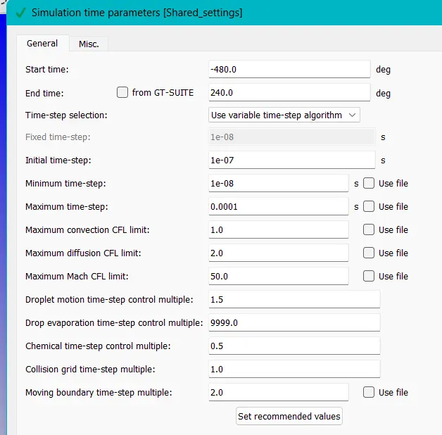
Simulation time parameters

1. Start time : -520 deg
2. end time : 120 deg

Boundary conditions

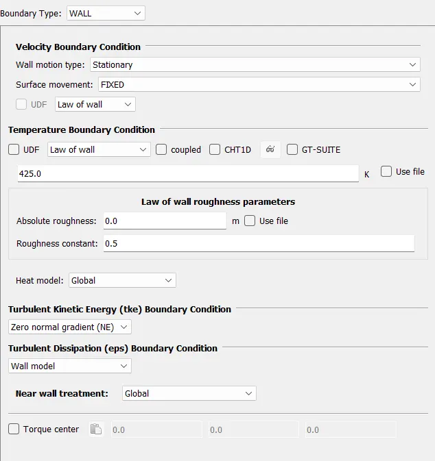
1. Piston temperature - 450K
2. Liner temperature - 450K
3. Head temperature - 450K
4. Spark Plug temperature - 550K
5. Spark Plug electrode temperature - 600K
6. Exhaust ports temperature - 500K
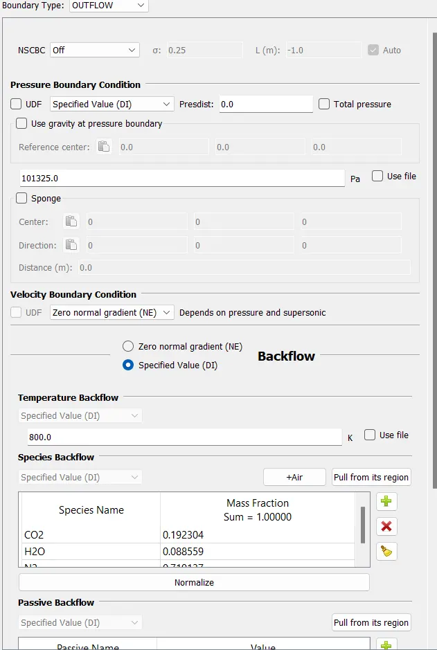
7. Exhaust outflow - 1 bar
8. Exhaust outflow temperature - 800k
9. Exhaust species concentration - Calculate the stoichiometric condition
10. Exhaust valve top temperature - 525K
11. Exhaust valve angle temperature - 525K
12. Exhaust valve bottom temperature - 525K
13. Intake port - 1 temperature 425K
14. Intake port - 2 temperature 425K
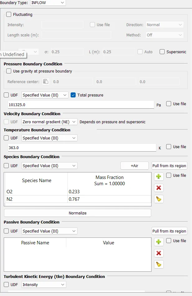
15. Inflow pressure - 1 bar total pressure
16. Inflow temperature - 363K
17. Inflow species - Air
18. Intake valve top temperature - 480K
19. Intake valve angle temperature - 480K
20. Intake valve bottom temperature - 480K

Initial conditions

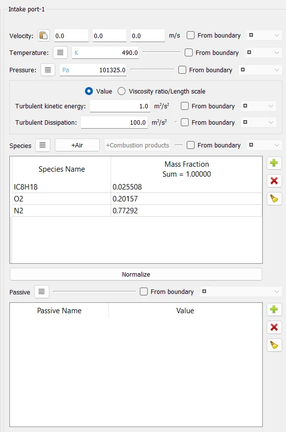
• Intake port - 1 (closer to combustion chamber)
  • ic8h18 - 0.025508
  • o2 - 0.20157
  • n2 - 0.77292
  • Temperature - 390k
  • pressure - 1 bar
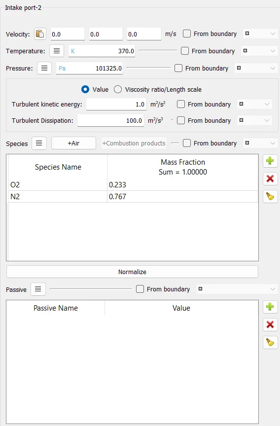
• Intake port - 2 (away from combustion chamber)
  • Air
  • Temperature - 370K
  • Pressure - 1 bar
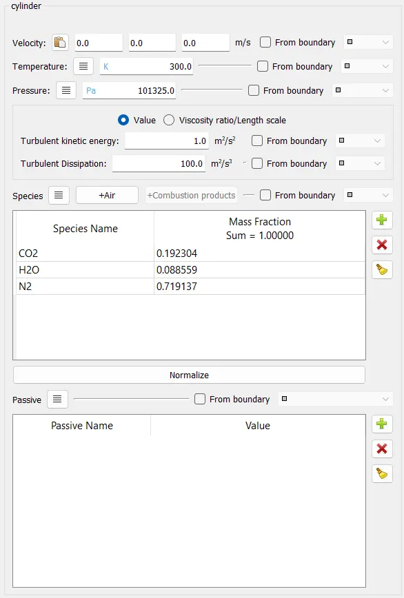
• Cylinder
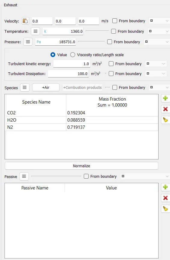
  • Pressure - 1.85731 bar
  • Temperature - 1360K
  • Stoichiometric composition

Injection Parameters

1. Fuel flow rate = 7.5e-4 Kg/second
2. Injection start time = -480.0
3. Injection duration = 191.2
4. Fuel temperature = 330K

Nozzle positions

Nozzle diameter = 250 micro-meter

Circular injection radius = Nozzle radius

Spray cone angle = 10

• Nozzle 0
  • center 0.0823357 0.00100001 0.07019
  • Align Vector -0.732501 0.210489 -0.647408
• Nozzle 1
  • center 0.0823357 -0.00099999 0.07019
  • Align Vector -0.732501 -0.210489 -0.647408
• Nozzle 2
  • center 0.0823357 -0.0004 0.07019
  • Align Vector -0.5 -0.2 -0.647408
• Nozzle 3
  • center 0.0823357 0.0003 0.07019
  • Align Vector -0.5 0.2 -0.647408

Spark Ignition Parameters

• Start of spark = -15 deg
• Spark duration = 10 deg
• Spark location = -0.003 0 0.0091
• Spark radius = 0.0005m

Objectives:

1. What is the compression ratio of this engine?

2. Why do we need a wall heat transfer model? Why can't we predict the wall temperature from the CFD simulation?

3. Calculate the combustion efficiency of this engine

4. use the engine performance calculator, to determine the power and torque for this engine.

Since Work and Torque has the same unit (N-m), it doesn't mean value for Torque and Work will be the same.

Both are different quantities and has totally different meaning.

So the value for work that you will be getting from the engine performance calculator is not the value for the torque.

Calculate the value for the torque using the formula as shown below,

Power(P) = (2*π*N*T)/60

5. What is the significance of ca10, ca50 and ca90?

Description:

Port Fuel Injection (PFI) is a type of fuel injection system commonly used in modern internal combustion engines. It involves delivering fuel directly into the intake ports of each cylinder, providing precise control over the air-fuel mixture. This technology has significantly improved fuel efficiency, power output, and emissions reduction compared to older carburetor systems.

The main feature of the PFI is that fuel is injected into the intake tract, PFI is stable and reliable, with low injection pressure requirements and more sufficient time for fuel and air to mix, but this approach has low delivery efficiency, cannot achieve precise fuel control, and most critically, is difficult to overcome the impact of low hydrogen bulk density on engine performance and the risk of backfire.

PFI is the most basic and straightforward EHCP technique for reducing NOx emissions. Port fuel injectors are located closer to the intake valve, which is located at the engine's intake port or manifold. The injection of fuel starts during the suction cycle and is permitted with air in the engine cylinder, causing disorder in the engine cylinders and helping to form a charge. However, the poor mixing of high and low unstable fuels leads to high emissions of UHC and PM. This makes it recommended to use port fuel injection for low-viscosity and highly unstable fuel such as alcohols and petrol. Higher in-cylinder or high intake charge temperature can improve fuel vaporization through prewarming of low unpredictable fuel and high thick fuel, yet just with a part load. The rich air-fuel mixture is recommended to obtain required output power at higher operating load conditions. Therefore it is difficult to form homogeneous charge with low injection pressure at higher operating load conditions. It brings out inflated charge consumption and fundamentally builds outflow levels. Broad fuel infusion procedures are important to defeat the impediments of the HCCI engine utilizing PFI techniques.

Procedure:

Geometry cleanup:

Import the given model into converge GUI.

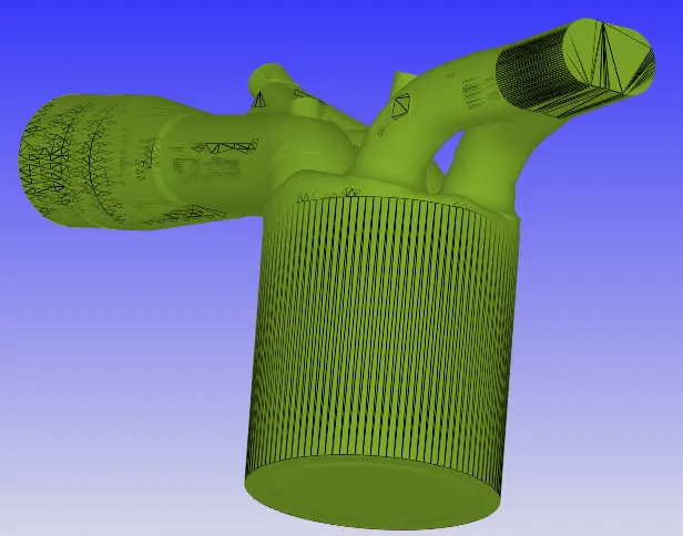
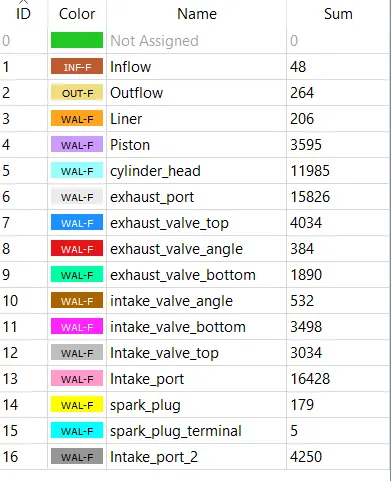
After, that flag the boundaries to the respective boundary regions.

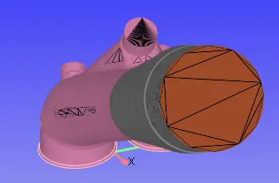
Inflow boundary:

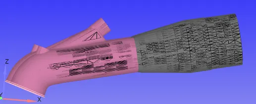
Intake port 1 and 2:

Here, the intake port is separated as Intale_port_1 and Intake_port_2. By using the boundary fence tool, the boundaries are flagged separately

Outflow Boundary:

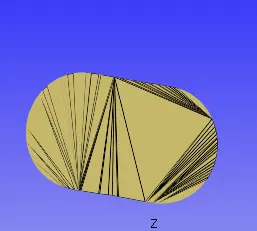
Exhaust port:

The entire exhaust port is flagged as exhaust port boundary.

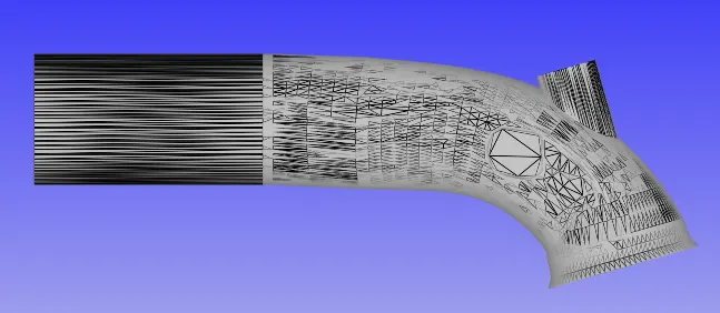
Liner:

The liner is the cylinder outer wall surface boundary.

Piston:

And the piston head surface is flagged as the piston boundary.

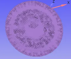
Cylinder head:

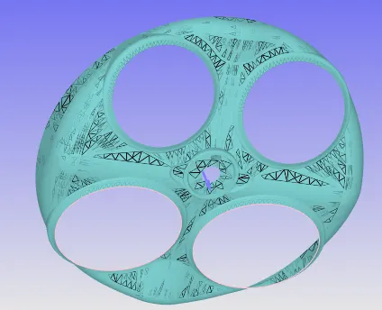
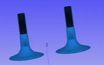
Exhaust valve top, bottom and valve angle:

The exhaust valve top, bottom, and valve angle surface are separated by using boundary fences and then flagged respectively.

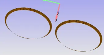
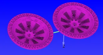
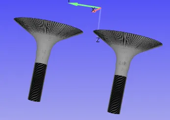
Intake valve top, bottom, and angle:

The intake valve top, bottom, and valve angle surface are separated by using boundary fences and then flagged respectively.

Spark plug:

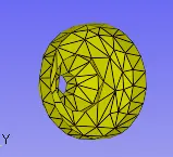
Spark plug terminal:

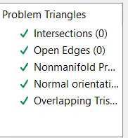
After, flagging the boundaries, check the diagnosis tool to identify the geometry errors like intersection, nonmanifold errors, normal orientation errors and so on. And here the diagnosis results no geometry errors.

Case setup:

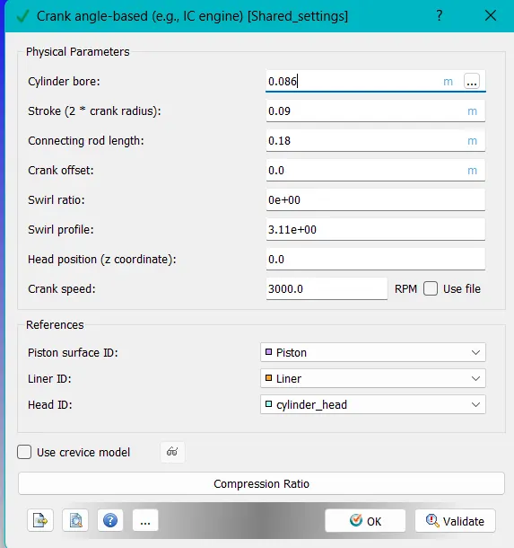
Application type: Crank angle -based

Here, the physical parameters of our ic_engine model are specified.

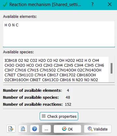
Reaction mechanism:

The given mech.dat data file is imported into here, and

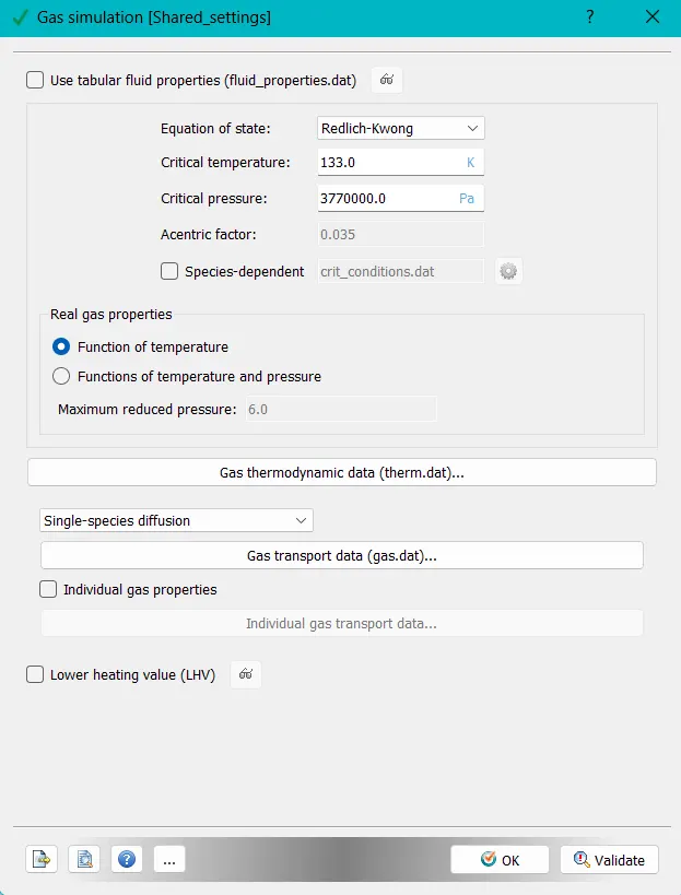
Gas simulation:

Here, the default values are taken under consideration

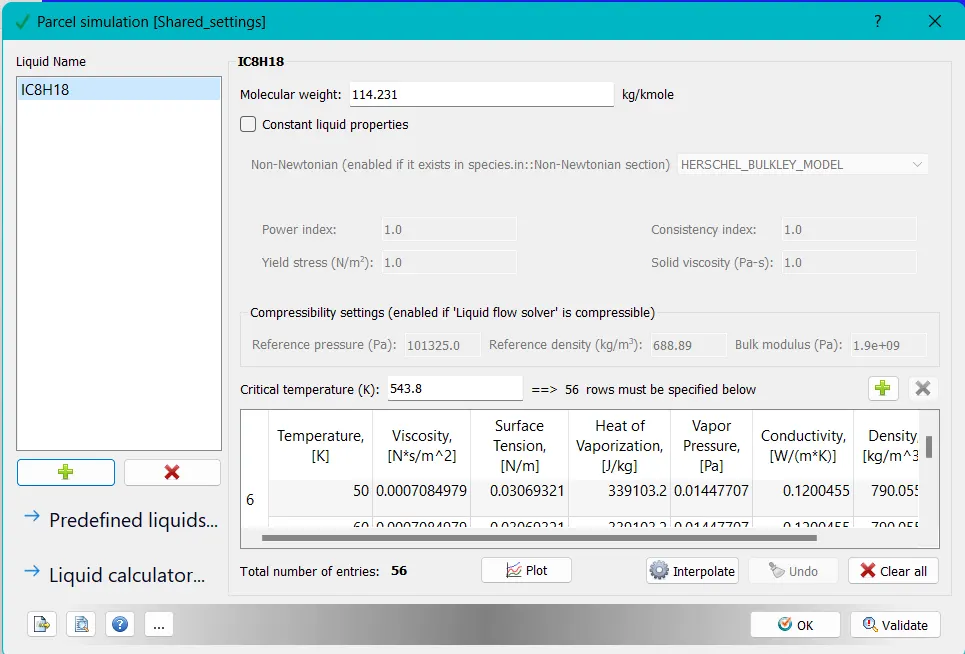
Parcel simulation:

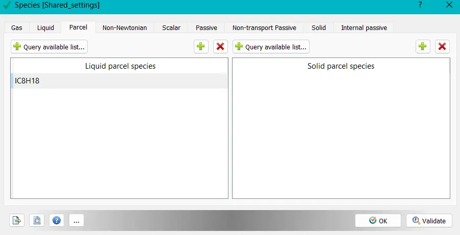
Here, fuel IC8H18 is selected from an available list of predefined liquid parcels.

Species:

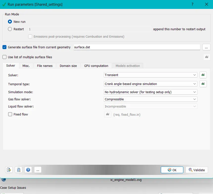
Run parameters:

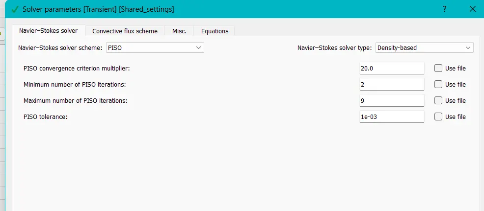
This case setup is solving under Transient solver, under no hydrodynamic solver simulation mode.

Simulation time parameters:

Solver parameters:

Boundary:

Inflow: region --> intake_port-2

Outflow: region --> Exhaust

Liner: region --> cylinder

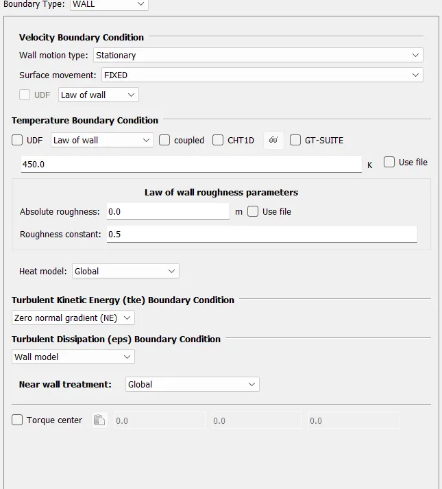
Piston: region--> cylinder

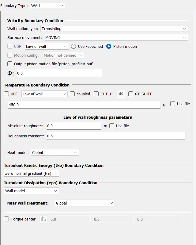
Cylinder head: region--> cylinder

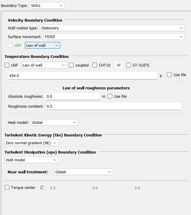
Exhaust port: region--> exhaust

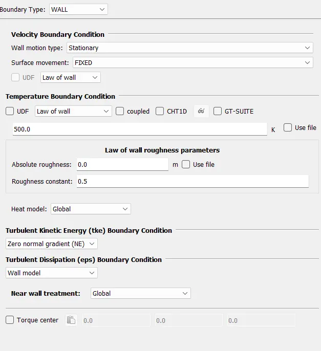
Exhaust valve top, angle: region --> exhaust

Exhaust valve bottom: region --> cylinder

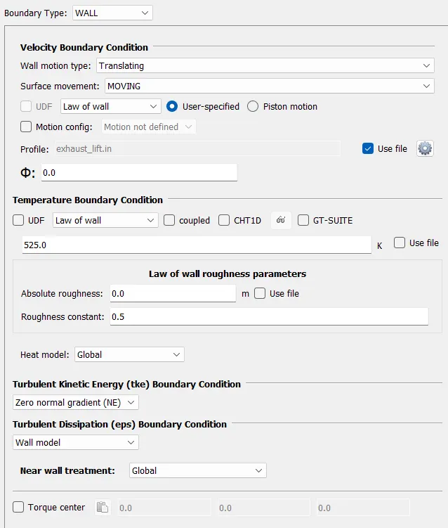
Intake valve angle, top: Region --> intake port-1

intake valve bottom: region --> cylinder

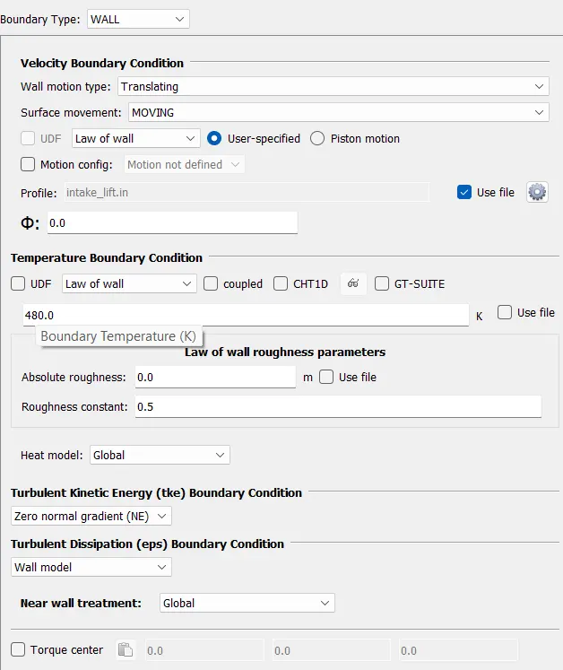
Intake port: region --> intake port-1

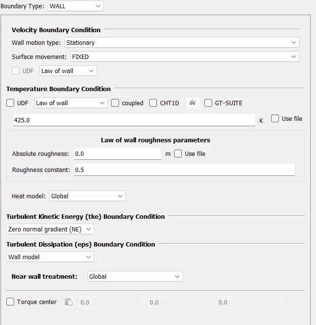
spark plug and terminal : region --> cylinder

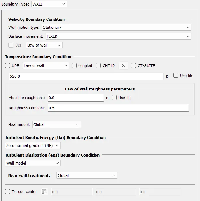
Intake port-2: region --> intake port -2

Regions and initialization:

cylinder:

Intake port-1:

Intake port-2:

Exhaust:

Events:

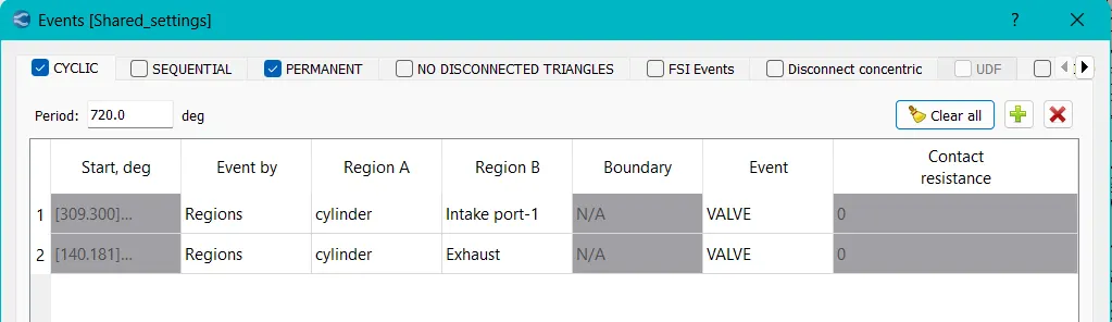
Cyclic:

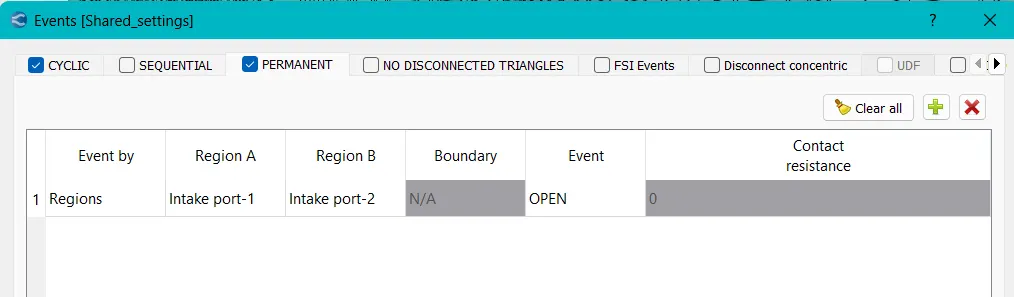
Permanent:

Physical Modeling:

• Parcel configuration:
  
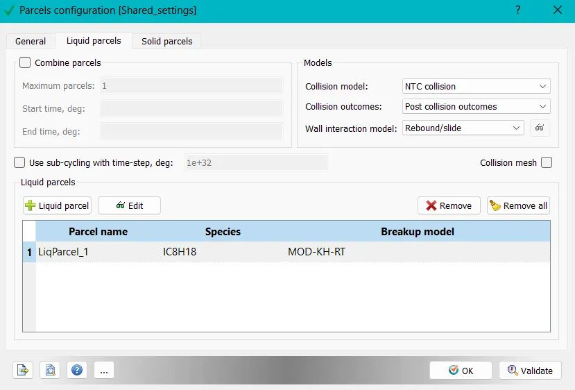
  The liquid parcel is loaded into this model under NTC collision model, which is used to describe the collision behavior of fuel particles through elastic collisions.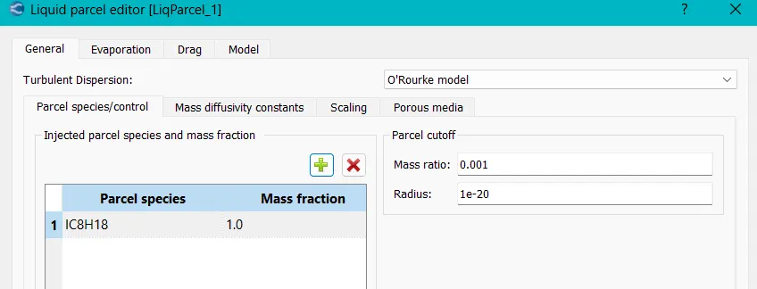
  
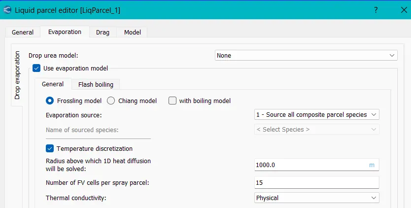
  O’Rourke model in Turbulent Dispersion is for Gasoline, and it used to analyze how turbulence affects droplet characteristics. And the evaporation model is used to capture the rate at which the parcel radius is going to change.
  
• Parcel Introduction:
  
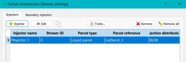
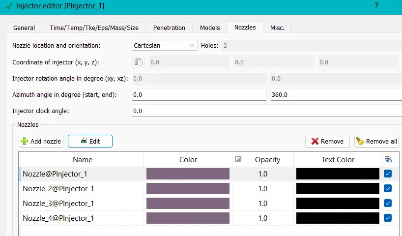
  Here, the spray injector is placed with 4 nozzle setup by specifying their characteristics, and under cyclic conditions.
• Combustion modelling:
  
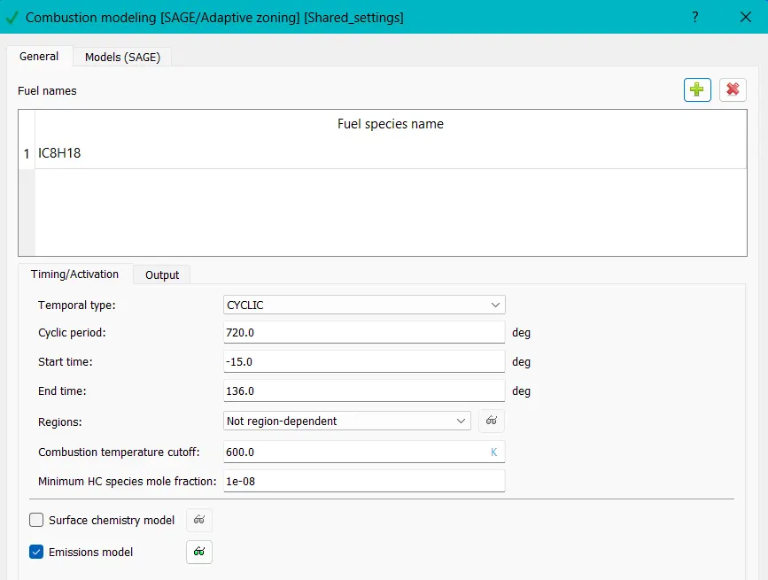
  The fuel species are specified under combustion timing conditions, and to accurately predict the ignition as well as turbulent frame propagation SAGE model is applied.
• Emissions modelling:
  To predict the emission particles production during combustion, Nox model is applied under equilibrium conditions.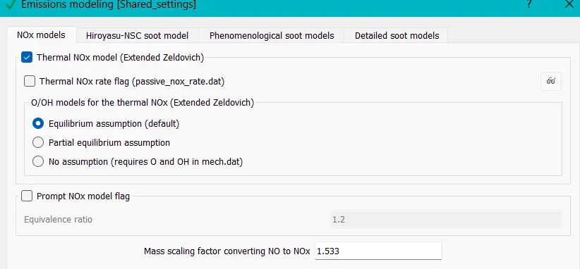
  
  
• Source/sink modeling:
  
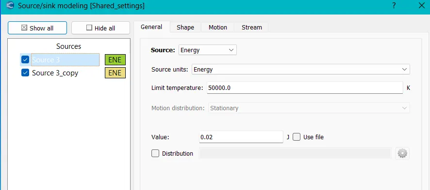
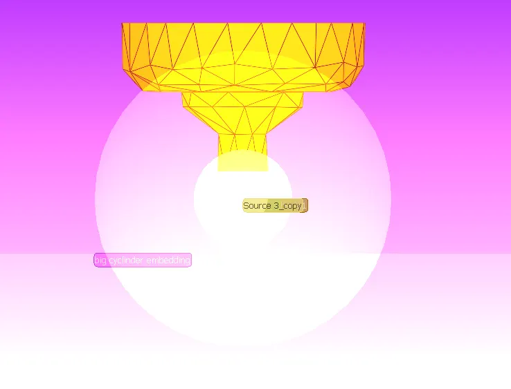
  Two heat source sphere are created and are discretized into cells, and inside the sphere temperature is constant in a cycle mode, and starts at -15 degrees, and thus acts like a energy source at the spark terminal. Total 0.04J of energy is created by using two sphere sources

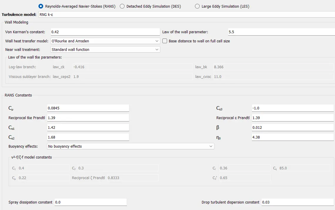
Turbulence modeling:

Base Grid:

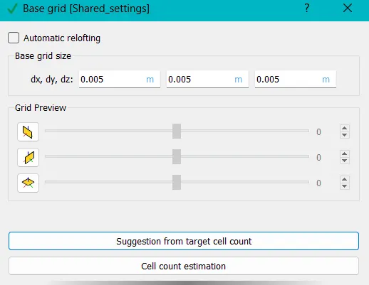
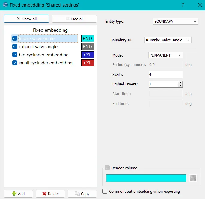
Fixed Embedding:

Intake valve angle and exhaust valve angle:

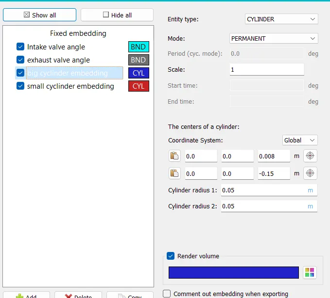
Big cylinder embedding:

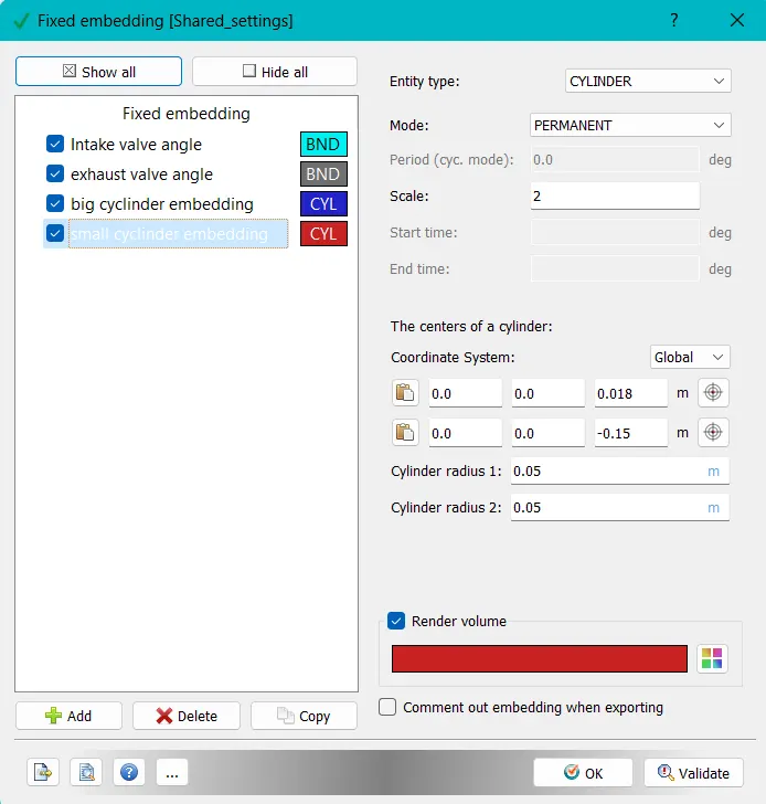
Small cylinder embedding:

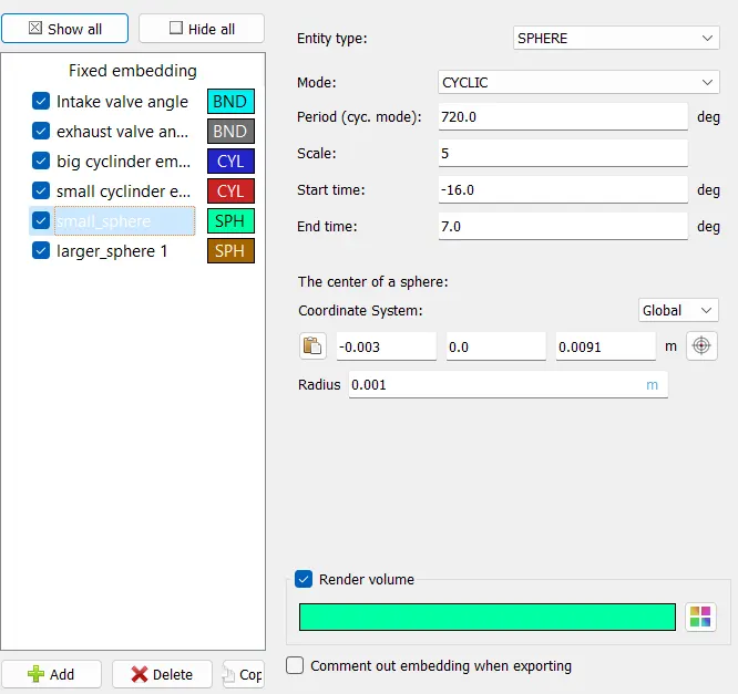
Small sphere:

Large sphere:

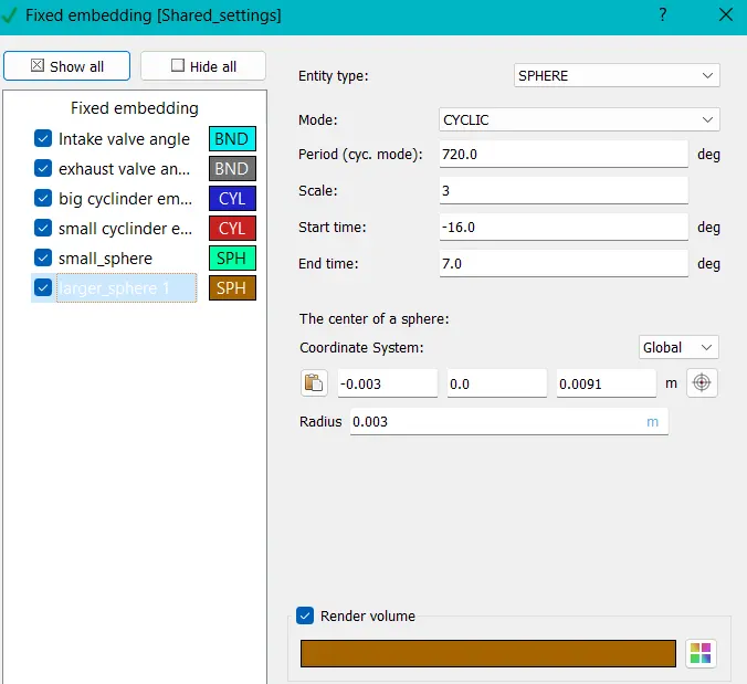
And the small and large spheres are embedded by scale 3 and 4 respectively.

Output files:

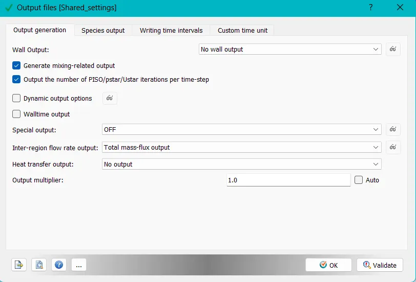
After validating the case set up, the input files are exported into the test case folder (File --> Export --> Export input files).

Running the Simulation:

• Open cygwin and navigate into the case directory where we exported the case setup input files.
• Run the following command
  $ mpiexec -n 4 converge --license explore
  
• This commands checks the license and converges the test case and generates output files.
• The to post process the results in Paraview, the output files are converted into group file format that supports in paraview.
• Then load the converted file into paraview to post process the results.

Post-Processing Results:

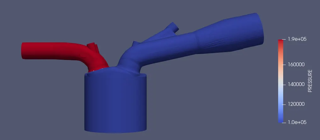
Pressure contour:

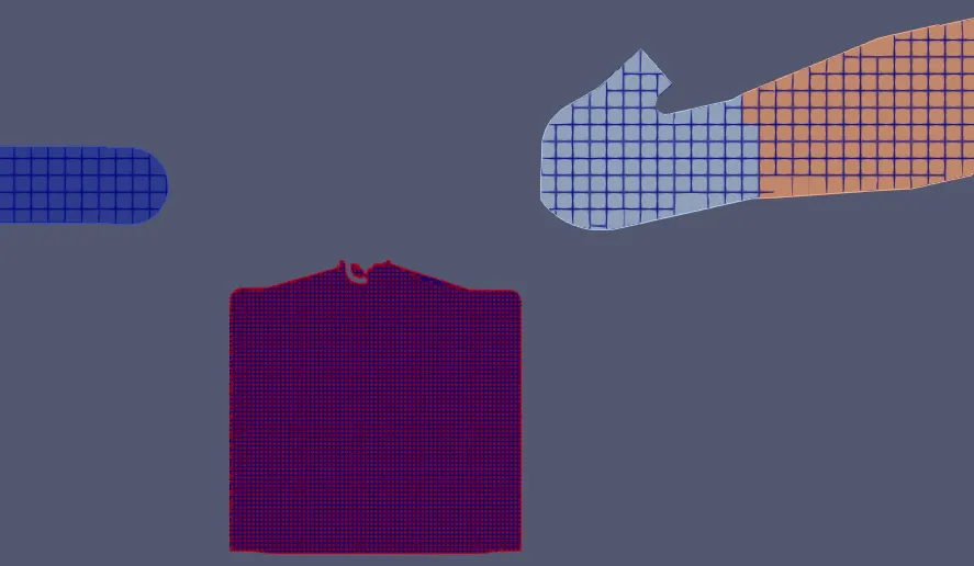
Mesh results:

Temperature contour animation: https://youtu.be/uhdQ76nHs3c

spray formation: https://youtu.be/r0bolWGigm8

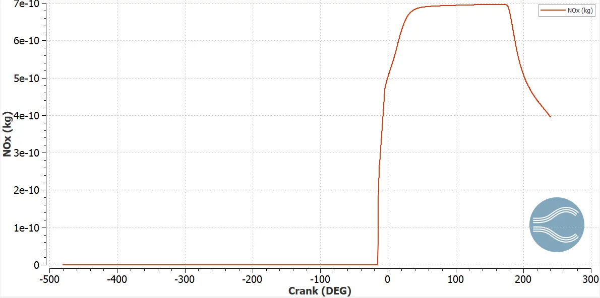
Nox emission plot wrt crank angle:

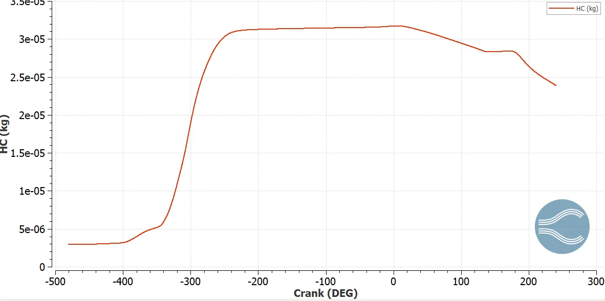
Hc emission plots wrt crank angle:

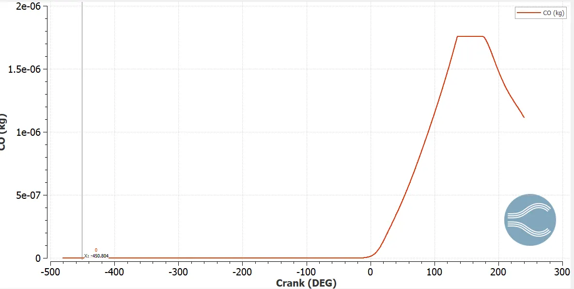
Co emission plots wrt crank angle:

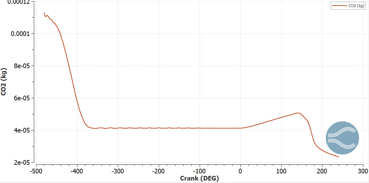
Co2 emission plot wrt crank angle:

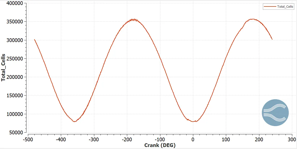
Total cells generated:

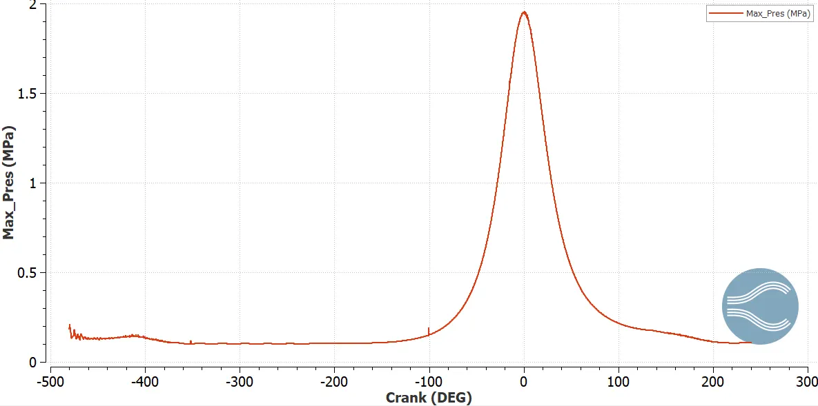
max pressure:

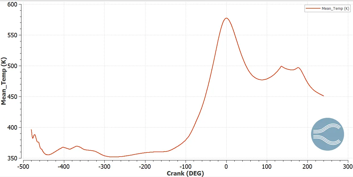
Mean temperature:

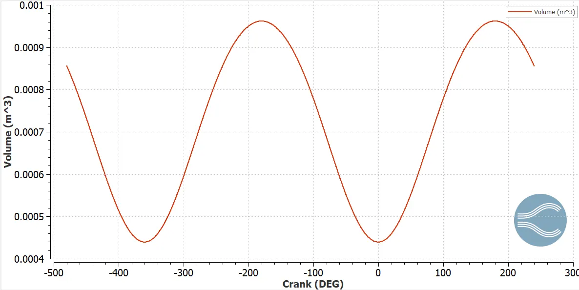
volume:

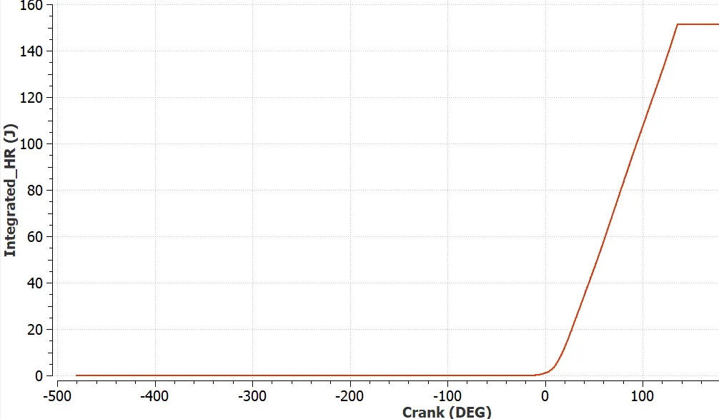
Integrated heat:

1. What is the compression ratio of this engine?

Compression ratio is defined as the ratio of maximum volume of the cylinder to the minimum volume. Where the maximum volume is the volume when the piston is at its bottom dead center (BDC), and the minimum volume is the volume when the piston is at its top dead center (TDC).

Compression ratio = (Maximum volume) / (Minimum volume)

The Compression ratio (rc)of an engine is the ratio of total cylinder volume to the clearance volume.

rc= (Vs+Vc)/(Vc) = 1+(Vs/Vc)

where Vs = Stroke volume = 5.2 x 10-4 m3

Vc= Clearance volume = 5.5 x 10-5 m3

rc= 1+(Vs/Vc) = 1+(5.2 x 10-4 / 5.5 x 10-5 ) = 10.45

2. Why do we need a wall heat transfer model? Why can't we predict the wall temperature from the CFD simulation?

Wall heat transfer models are essential in Computational Fluid Dynamics (CFD) simulations to accurately predict the temperature distribution and heat flux at the solid-fluid interface. This information is crucial for understanding a wide range of engineering applications like

• Determining the effectiveness of heat transfer between fluids in Heat exchangers.
  
• Analyzing heat transfer to the cylinder walls and piston in ic engine simulations.
  
• Predicting the temperature of components to prevent overheating in Electronic applications.
  

While CFD simulations can provide detailed information about fluid flow and temperature fields, directly predicting the wall temperature can be challenging. Basically the wall temperature is often specified as a boundary condition in CFD simulations, this means the simulation assumes a known wall temperature and calculates the heat transfer to the fluid. While this approach is valid in many cases, it may not accurately capture the real-world scenario where the wall temperature is influenced by factors like external heat sources, conduction within the solid, and radiation. And also the factors like thermal conductivity of the wall material significantly affects heat transfer if the wall material properties are not accurately represented in the CFD simulation, the predicted wall temperature may be inaccurate. And also the wall surface roughness can influence heat transfer by altering the flow pattern near the wall.

3. Calculate the combustion efficiency of this engine

Combustion efficiency is a measure of how effectively the fuel is converted into useful mechanical energy in an internal combustion engine. It can be calculated using the following formula:

Combustion Efficiency (%) = (Actual Heat Released / Theoretical Heat Release) x 100

Actual Heat Realeased: This is the amount of heat generated during the combustion process. It is taken from Integrated heat release graph as 1244.1 J

Theoretical heat release = (LHV of fuel)*(mass of fuel consumed)

LHV of isooctane = 44.4 MJ/k = 44.4 x 106 J

mass of fuel consumed = 3x10^-5 Kg

Therefore, Combustion efficiency = 1244.1 /(44.4 x 106 )*( 3x10-5 ) *100 = 96.2%

4. use the engine performance calculator, to determine the power and torque for this engine.

Power is the rate at which work is done. In the context of an engine, it represents the rate at which the engine can convert chemical energy from fuel into mechanical energy.

power = work done / combustion time

Torque is a rotational force that causes an object to rotate around an axis. In an engine, it is the twisting force produced by the pistons.

Torque = (power*60)/ (2*π*N)

From the engine performance data

Gross work = 33.0979 N*m

Total combustion duration = 360.128 degree

engine speed = 3000RPM = 50RPS = 18000 degree/sec

so combustion time = 360.128/18000 = 0.02sec

Power = 33.0979 /0.02 = 1654w

Torque = (1654*60)/(2*π*3000) = 5.26 N-m

5. What is the significance of ca10, ca50 and ca90?

The ca10 ca50 and ca100 defines the positions of crank angle at which the net heat release facter reaches 10%, 50% and 100% respectively. This signifies the rate of ignition and diffusion rate in an engine. Higher the difference between ca10 and ca50, more the combusion time and vice versa.

Conclusion:

In this report a full hydro simulation of PFI engine model is performed by setting up the combustion and Emission models. And the mesh is properly refined by using AMR, and Fixed embedding tools. Then post-processed the animation results and graphical plots are studied and calculated the engine performance parameters and examined the emission results.