Week 10: Project 1 - FULL HYDRO case set up (PFI)
Week 10: Project 1 - FULL HYDRO case set up (PFI)
AIM: -
To run the full hydro simulation in the Single-cylinder four-stroke gasoline engine with a port fuel injection system using Converge 3.0 Software.
INTRODUCTION: -
In this full hydro simulation, the previous no hydro simulation set up is taken and convert into the full hydro simulation spray modeling, combustion modeling and source, sink modeling processes are completed for the simulation of the gasoline engine with port fuel injection system. The innovative approaches from the converge 3.0 basic grid 0.004m is fixed including that adaptive mesh refinement modeling and fixed embedding modeling are given the best contour plots in the simulation process.
PROGRESS: -
Step 1: Upload from the 3D modeling, surface preparation and boundary flagging is completed in the previous challenge.
Step 2: After the previous challenge, first of all, add the parcel simulation in the material selection case set up and choose the predefined liquids to select the IC8H18 is similar to the gasoline fuel add to the parcel liquid material and click ok then done.
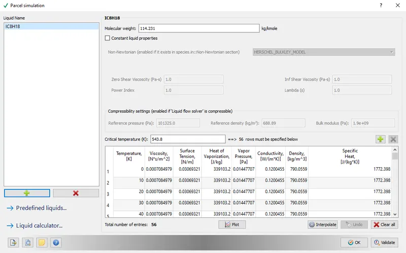
Figure: predefined Liquid added to the parcel simulation set up
Step 3: For the material case set up select the species as IC8H18 as fuel and its added into the parcel region and click ok then done.
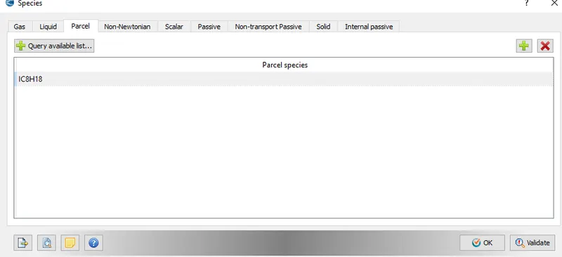
Figure: Fluid gasoline parcel added to the species section
Step 4: Next for the important boundary selection and region selections are all fix as per the previous no hydro surfaces preparation and boundary flagging techniques.
Step 5: Next for the physical model set up select the spray modelling and choose the distribute parcels evenly throughout the cone in the parcel distribution field. Also select the O’ Rourke model in the turbulent dispersion because of it’s the gasoline fuel engine.
Step 6: Next important set up is for the injector are fixed in the inlet port, add the injector in the injector case set up select the injector_0.
Step 7: Click the edit option for the injector set the configuration of the injector, in the required set up has 4 different positon nozzles added in the injector. First of all, the IC8H18 as the species parcel and set the mass fraction of the species is 1.0 and click ok then done.
Step 8: For the gasoline fuel spraying nozzle have the different type of model set up, so this nozzle has set for the two combined models selected as Kelvin- Helmholtz model + Rayleigh – Taylor model and also added the additional model as Discharge coefficient model and set the discharge coefficient value as 0.8 click to apply then done.
Step 9: From the design team development the injection temporal type is set as Cyclic and the total cyclic period is 720 degrees. Start of the injection is 480 degrees and injection duration as 191.2 degrees.
Step 10: For the fuel injected mass calculation,
- Speed: 3000 RPM
- Fuel mass / Cycle: 300e-5 kg/s
- Speed in RPS: 50
- Speed in DPS: 18000
- Time/ Degree: 55556e-5
- Time / 720 degree: 04
- Fuel flow rate: 50e-4
From the previous data’s Total inject mass is calculated as 3.0e-5 kg and the injected liquid temperature is set as 330 K.
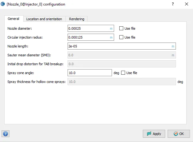
Figure: Nozzle injection configuration set up
Step 11: Next for the nozzle location set up select the option for Nozzle location and orientation is set as Cartesian coordinates and that add all the 4 nozzles and click edit option set for the nozzle diameter is 0.00025 m, circular injection radius is 0.000125 m and the nozzle length set as 2e-5 m and that the spray cone angle is 10 degrees.
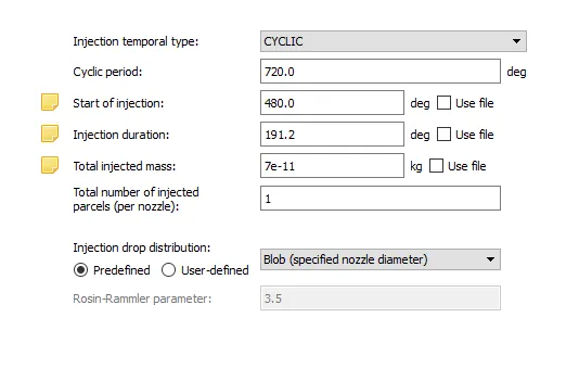
Figure: Injection nozzle coordinate set up
Step 12: The location of each four nozzle set as below,
For the nozzle 1:
Coordinate of the Nozzle (x, y, z): x=0.0823357 y=0.00100001 z=0.07019
Spray orientation vector (x, y, z): x=-0.732501 y=0.210489 z=-0.647408
For the nozzle 2:
Coordinate of the Nozzle (x, y, z): x=0.0823357 y= -0.00099999 z= 0.07015
Spray orientation vector (x, y, z): x=-0.732501 y=0.210489 z=-0.647408
For the nozzle 3:
Coordinate of the Nozzle (x, y, z): x=0.0823357 y= -0.0004 z=0.07019
Spray orientation vector (x, y, z): x=-0.5 y=0.2 z=-0.647408
For the nozzle 4:
Coordinate of the Nozzle (x, y, z): x=0.0823357 y=0.0003 z=0.07019
Spray orientation vector (x, y, z): x=-0.5 y=0.2 z=-0.647408
Step 13: Next set up for the physical model is combustion modeling, set as this model named as SAGE, Fuel species name is set as IC8h18 and the temporal type is Cyclic, the cyclic period is 720 degrees, start time is -17 degree, End time is End time 130 degree and the combustion temperature cutoff is 600 K.
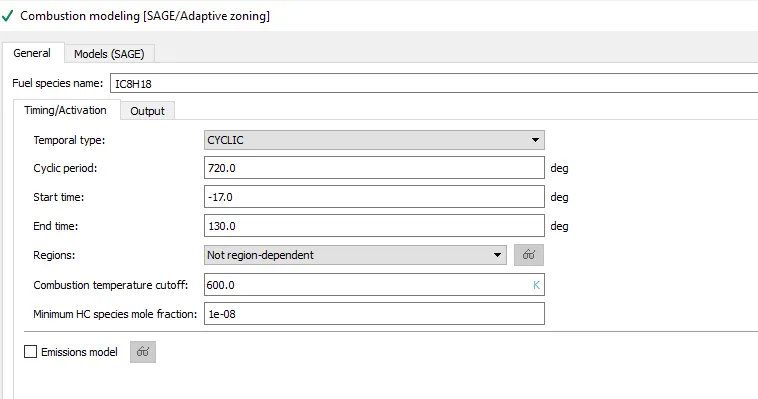
Figure: Combustion modeling set up configuration
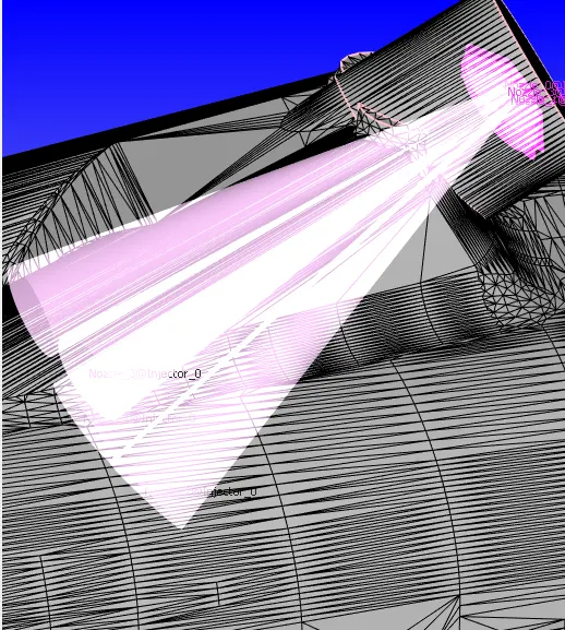
Figure: Four nozzles fixed in the inlet port of the Engine
Step 14: Next for the source and sink modeling, this modeling is set for the intermediate location of the spark plug terminal, so to fix the shape this source and sink modeling is used. For that modeling add the source shape is the sphere and the location of the sphere is x= -0.003 y= 0.0 z=0.0091 and fixed the sphere radius is 0.0005 m.
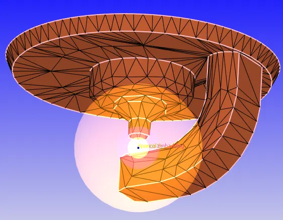
Figure: create the Spark plug terminal set up used in source-sink modeling
Step 15: Using the fixed embedding option, create the mesh refinement in the spark plug terminal add the two different spherical fixed embeddings in the intake valve angle boundary.
Step 16: Also create the injector embedding entity type is an injector, the period is 720-degree scale is 4, The start time is -482.0 deg, End time is -286.0 deg set the position of the injector Radius 1 is 0.002 m radius 2 is 0.004 m length is 0.002 m.
Step 17: After finishing the process and case set up the surface preparation, boundary flagging and full hydro set up of the gasoline engine model is shown below.
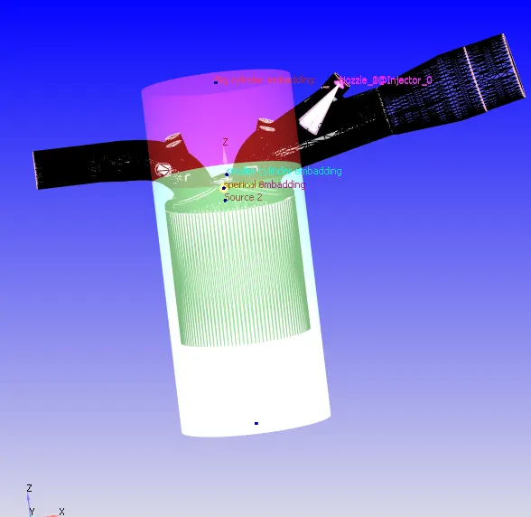
Figure: Surface preparation and boundary flagging and full hydro set up of the engine
RESULT AND DISCUSSION: -
In this gasoline is mixed with air, broken up into a mist and partially vaporized in a carburetor. The mixture is then sucked into the cylinder. There it is compressed by the upward movement of the piston and is ignited by an electric spark. When the mixture is burned, the resulting heat causes the gases to expand. The expanding gases exert a pressure on the piston (power stroke). The exhaust gases escape in the next upward movement of the piston. The strokes are similar to those discussed under four-stroke diesel engines. The various temperatures and pressures are shown in Fig. 6. The compression ratio varies from 4:1 to 8:1 and the air-fuel mixture from 10:1 to 20:1.
- What is the compression ratio of this engine?
The maximum volume of the combustion chamber (with the piston farthest out, or bottom dead center) divided by the volume with the piston in the full-compression position (with the piston nearest the head of the cylinder, or top dead center).
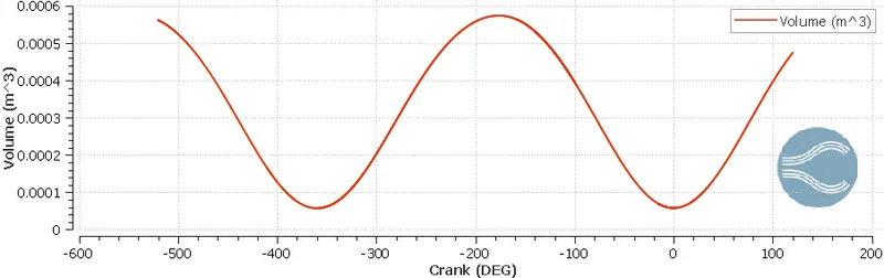
Figure: Crank angle vs Volume
From the graph,
The maximum volume of the engine is: 0.0005742195 at 176.2 degree
The minimum volume of the engine is: 0.000057539186 at -7 degree
The compression ratio of the engine is: Maximum volume / Minimum volume
= 0.0005742195 / 0.000057539186
Compression ratio = 9.98
- Why do we need a wall heat transfer model?
Several assumptions are introduced in the derivation of the model, including the following: (1) fluid velocity near walls is parallel to the wall, and only the temperature and density gradients normal to the wall are considered, (2) the gas is assumed to be ideal, (3) the pressure is uniform in space, (4) viscous dissipation is neglected, and (5) radiation heat transfer is not included.
In order to perform good prediction of engine heat transfer and wall temperature, models are required for accomplish heat transfer from hot gases to engine parts, heat transfer inside each engine part, and also heat transfer to coolant and lubricating oil.
- Why can't we predict the wall temperature from the CFD simulation?
For the PFI Engine simulation it takes lot of time to compute the case as it contains complex geometry. For this if we want to compute the heat transfer we need to solve energy equations to get convection of heat from liquid solid surface. Thus it difficult to take wall temperature for cfd simulation.
A mesh independency study only eliminates - if carefully carried out - the numerical errors from the CFD solution, like there are the round-off error, the iteration error and the discretization errors in space and time.
But what finally a mesh independency study cannot eliminate or help to quantify is the remaining model error. After doing it, nobody could tell whether for example the CFD result with a k-epsilon turbulence model or a SST turbulence model or a LES is the more accurate one. This can only be found out and be quantified, if the different CFD results are compared to real-world, i.e. experimental data.
That a thorough literature search will reveal some experimental data about convective heat transfer for a heated cylindrical body. It is quite a generic test case which most likely has already been studied in the past. I have the paper not to my disposal, but I did such a validation study already by myself with a Master student and there were some Nusselt number distribution over the cylinder surface for comparison.
- Calculate the combustion efficiency of this engine.
The combustion efficiency ηc [-] is defined as the ratio between the energy released by the burnt fuel and the theoretical energy content of the fuel mass during one complete engine cycle.
ηc = Brake power / (Cv * mf)
Here ηc = Combustion efficiency of the engine
Cv = Calorific value of fuel J/kg - K
mf = mass of fuel supplied kg/s
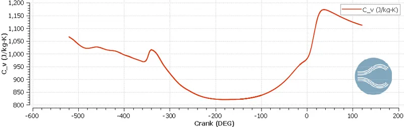
Figure Crank angle vs Cv (J/kg- K)
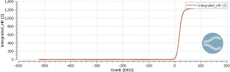
Figure: Crank angle vs Brake power (Integrated Heat Release)
From the graph and previous input values,
Cv = 44000 KJ/kg
mf = 3 e-5 kg
BP = 1241 J
ηc = Combustion efficiency of the engine = 1241 / (3e-5 * 44000) = 0.94 = 94%
Combustion efficiency of the engine = ηc = 94%
- Use the engine performance calculator, to determine the power and torque for this engine.
To attain the engine performance calculator à click the line plotting module of the Converge 3.0 à click tools à Engine calculator àEngine performance
First of all, Cycle interval is set as half cycle 3600 and click option as add file à add thermoregion0.out file à upload it will get the Start and end crank angle and total duration of crank angle.
Next click the Load from engine.in option and add the engine.in file from the exporting input file for the gasoline engine in the full hydro simulation model.
Get the Stroke is 0.0900 m and bore = 0.0860 m after that click the calculate option will get the all the output details of the engine performance.
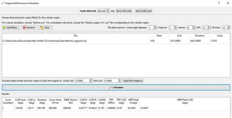
Figure: Engine performance calculator
To calculate the power of the given engine: -
Power = Work/sec
Work from the engine performance calculator = 486.646 Nm
Total duration = 240.2 degree
Total RPM = 3000 (from previous calculation)
Dps = 18000
Time in sec = 240.2/18000 = 0.01334 sec
Power = 486.646/0.01334 = 35130.22 W = 35.13 KW
Torque calculation: -
Power = 2 π NT / 60
T = Power * 60 / 2 π N
T = 35130.22 * 60 / 2*3.14* 3000 = 111.879 Nm
- What is the significance of ca10, ca50 and ca90?
The physical significance of CA10 is that it is used to identify the start of ignition in an engine, whereas the CA50 indicates the end of premixed combustion and the start of diffusion combustion of fuel used in the engine. The CA90 indicates the end of exhaust process of the engine.
Figure: The significance of the CA10, CA50 and CA90
CA10 occurs: 6.83717 degree
CA50 occurs: 18.4623 degree
CA90 occurs: 37.701 degree
Liquid spray parcel at the inlet region (thermoregion0.out): -
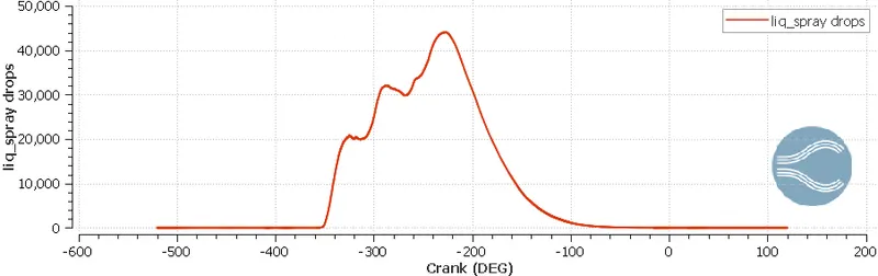
Figure: Crank angle vs Liquid spray parcel (inlet region)
Liquid spray parcel at the exhaust region (thermoregion3.out)
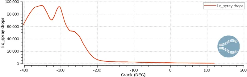
Figure: Crank angle vs Liquid spray parcel (Exhaust region)
Fuel consumption: -
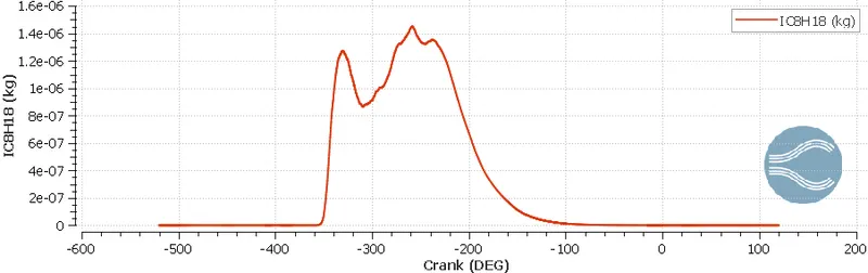
Figure: Crank angle vs Fuel consumption
Emission characteristics of the engine: -
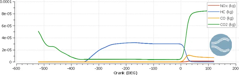
Figure: Crank angle vs various emission occurs in Engine
CONCLUSION: -
The simulation of the single cylinder four stroke gasoline engine with port fuel injection completed with converge 3.0 software. Also analyzed the performance and emission characteristics of the engine. The efficiency of the engine is calculated as 90% and the torque of the engine is 111.879 Nm. The compression ratio of the engine is also calculated as 9.98.
YouTube Video Link: - https://youtu.be/tTyRL2wiimU