Week 10: Project 1 - FULL HYDRO case set up (PFI)

AIM: FULL HYDRO case set up of port fuel injection for IC engine.

OBJECTIVE:

• Simulate the SI engine using Converge CFD software and discuss the results.
• Calculate engine performance parameters such that we can make design changes.

INTRODUCTION:

Spray modelling:

• Converge can model both gaseous and liquid sprays.
• Converge includes state-of-the-art models for spray processes including liquid atomization, drop breakup, collision, and coalescence, turbulent dispersion, and drop evaporation.
• The spray model is a simplified mathematical model to capture the approximate behavior of the spray.

Gaseous and liquid spray modelling techniques:

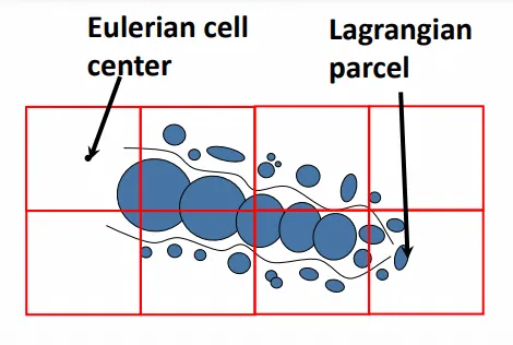
• For gaseous sprays converge uses the Eulerian solver.
• For liquid sprays converge uses the Langrangian solver to model discrete parcels and the Eulerian solver to model the continuous fluid models.

Parcels:

• Converge introduces parcels (Collection of drops) into the domain at the injector.
• Each parcel represents a group of identical drops (i.e. same radius, velocity, temperature, etc.).
• It solves for properties on a per-parcel basis rather than a per-drop basis (because parcels are identical).
• The parcels statistically represent an entire spray field.

Parcels undergo several physical processes:

• Primary breakup
• Secondary breakup
• Drop drag
• Collision and coalescence
• Turbulent dispersion
• Evaporation

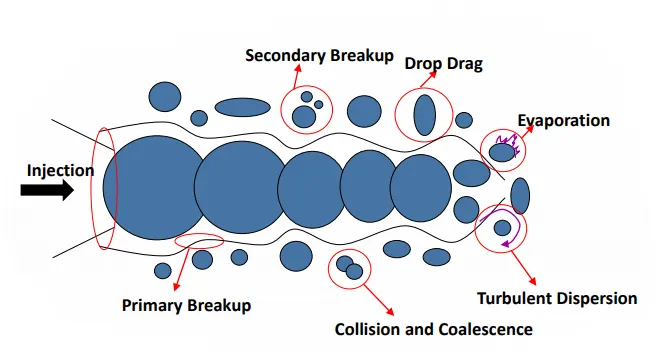
When the spray is injected due to internal drag force the primary and secondary breakup takes place, the parcel may change shape which will lead to fast evaporation or slow evaporation which results in the reduction of parcel size, and due to internal velocity there is turbulent dispersion also collision and combining of two parcels getting all these processes will lead to approximate spray modelling.

Sub-grid modelling setup

Go to setup -> physical model -> spray modelling

To set up parcels, go to case setup -> Materials -> Species -> Parcels

Parcel distribution:

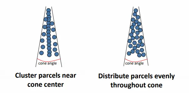
For solid cone sprays, converge assumes the injection is conical.

We can choose between two types of parcel distribution:

• Cluster parcel near cone center.
• Distribute parcels evenly throughout the cone.

Evaporation Model:

There are two models for evaporation modelling,

• Frossling model
• Chiang model

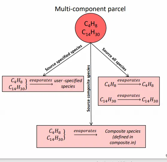
Evaporation source: since the liquid is evaporating there is extra gas mass which should be included as source terms in the model

Select evaporation source to specify how to converge simulate multi-component vaporization

The source specified species:

• Parcel evaporates to the specified species.

Source all-composite parcel species:

• If composites are defined, multi-component liquid species evaporate into composite species.
• If composites are not defined, multi-component liquid species evaporate into base species.

Source all base parcel species:

• Multicomponent liquid species evaporate into the base species.

Specify the maximum radius for ODE droplet heating which will control if the dropping temperature is non-uniform or radially varying.

If the drop doesn’t exceed the maximum value uniform distribution is assumed throughout the droplet, and if exceeds radially varying temperature distribution is assumed.

Spray penetration:

• Converge writes the liquid and vapor penetration lengths at each output interval specified in the case setup.
• Consider a control volume in which the liquid is injected, the length of injected liquid before vaporizing is called liquid penetration length.
• For liquid penetration length specify the liquid fuel mass fraction assume that we have injected ‘M_total ‘of mass the length at which we get ‘0.98*M­_total’ we assume that’s its liquid penetration length, this value can be set to any percentage of a mass fraction.

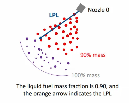
It is not calculated along the spray axis of the nozzle.

Converge calculates the liquid penetration length by calculating the fuel vapor mass fraction in each cell inside the spray cone.

For each cell that meets the below points converge calculates the distance from the center of the nozzle to the center of the cell.

1. The fuel vapor mass fraction exceeds the user-defined fuel vapor mass fraction (i.e. 1e-3 vapor in terms of the mass fraction)
2. The cell size does not exceed the user-defined bin size.

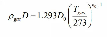
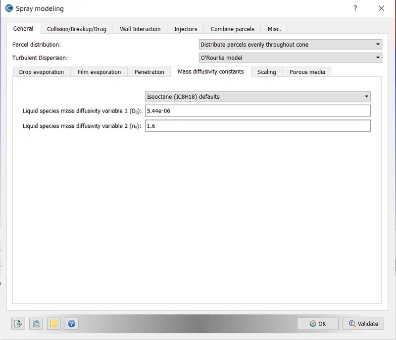
Mass diffusivity constant:

To calculate mass diffusivity of liquid vapor in the air.

Collision and Coalescence:

• Drop collision options
• No collision
• O’Rourke numerical algorithm
• NTC numerical algorithm

Collision mesh:

In typical spray, simulation parcels collide only with parcels of the same cell, which can lead to grid sensitivity.

In converge, we have an adaptive collision mesh option to reduce grid sensitivity.

Drop drag:

When a parcel enters through the gas space it encounters air resistance which causes the change of shape size and many other things inside the gas space.

The options for drop drag are:

• No drop drag.
• Spherical drop drag-

The drag co-efficient calculation assumes the drops are a perfect sphere.

• Dynamic drag model-

The drag co-efficient calculations account for variations in the drop shape.

This model invokes the TAB model to determine the drop distortion

Drop/wall interactions:

Rebound/slide:

Drops rebound or slide along the wall after impingement.

Wall film:

Drop actions are calculated with a hybrid approach based on particle-based quantities.

If we are using the wall film model we must select a film splash model.

O’rourke model:

Splash criteria based on the weber number, film thickness, and viscosity

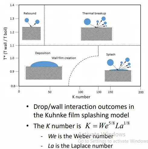
Kuhnke model:

The possible parcel outcomes are rebound splash, thermal breakup, or deposition.

Combustion modelling:

• Combustion facilitates the energy transfer in an engine.
• Converge contains a detailed chemistry solver and simplified combustion models

There are generally two types of combustion modelling techniques:

• SAGE modelling
• Simplified combustion modelling

SAGE:

• Sage detailed chemistry solver uses local conditions to calculate reaction rate based on principles of chemical kinetics.
• In each cell, we have different equivalence ratios, temperature, and pressure sage solver runs chemical kinetics reactions in each of the cells.
• The rate of change of species concentration is calculated using the Arrhenius rate equation.
• Converge consists of mechanism files in which detailed chemical reactions are provided which can be added manually by the users which can be used to calculate the Arrhenius rate equation.
• The rate of change of species concentration calculated using the Arrhenius rate equation is then substituted in the species transport equation and species mass fractions are calculated during the combustion process.

Arrhenius equation:

SAGE: Acceleration options-

• Solving detailed chemistry in every cell can be time-consuming.
• In converge we have options to reduce the computational time by increasing the minimum cell temperature and minimum HC species mole fraction to reduce the number of cells in which combustion calculations are performed.
• Using start-time and end-time to limit SAGE to a specific time interval.
• Limit SAGE to a particular region since we don’t want to solve for species mass fraction in intake and exhaust ports.
• Set resolve option to only resolve if temperature changes by specified temperature.
• Use iterative methods to pass analytically calculated values to the solver.

Acceleration options (Multi-zone model)-

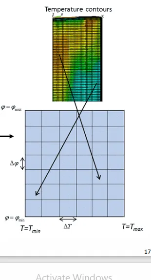
The multi-zone model reduces the number of SAGE calculations by,

• By grouping cells into bins (zones)
• The number of bins varies dynamically with the arrangement of the flow field parameters.
• Create bins based on two or more variables.

1. Equivalence ratio
2. Temperature
3. Pressure
4. Reaction rate

• Calculating average quantities.
• Invoking the SAGE solver once per bin instead of once per cell.

Other premixed turbulent combustion models:

• G-Equation
• Extended coherent flame model
• Chemical equilibrium (CEQ) model
• Flamelet generated manifold (FGM)

CASE setup:

Application type – Crank angle based IC engine

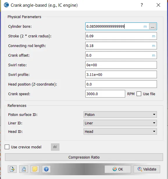
Physical parameters-

Cylinder bore: 0.086m

Stroke: 0.09m

Connecting rod length: 0.18

Crank speed: 3000

We should also select a reference Id for the references mentioned in the setup

Materials:

Gas simulation: Same as that of no hydro simulation (providing therm.dat file for including all the reaction species).

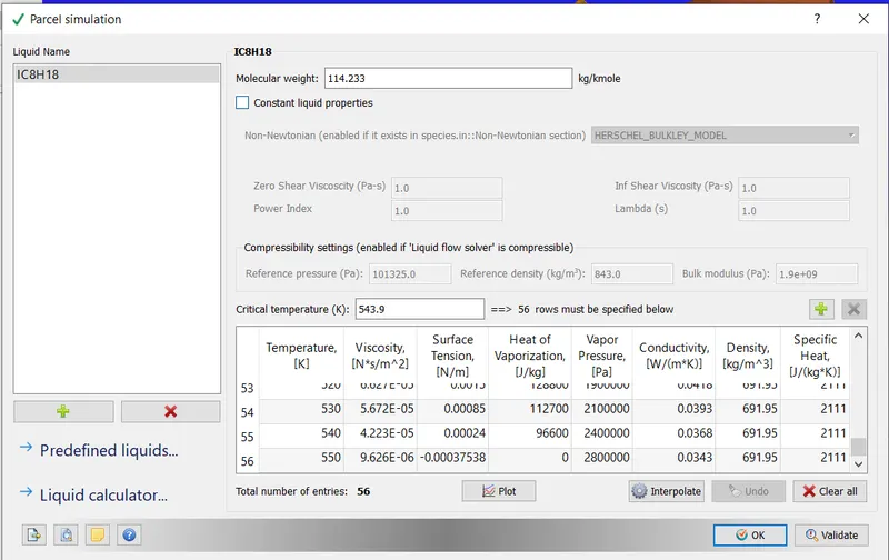
Parcel simulation:

Add pre-defined liquids we will be using iso-octane as our fuel select it, all the properties of fuel at a different temperature will be included (i.e. viscosity, surface tension, density, etc.).

Reaction mechanism:

Add mech.dat file which consists of mechanisms for our fuel and validate.

Species:

Under parcel, we should add our fuel species (iso-octane).

Simulation parameters:

Run parameters:

Solver: Transient

Temporal type: crank angle based engine simulation

Mode: Full hydrodynamic

Gas flow solver: compressible

Boundary conditions:

Piston:

Type: Wall, translating, and moving

Piston temperature - 450K

Liner, Head, spark plug, spark plug electrode, Exhaust port, Intake port, and intake port B:

Type: Wall, stationary and fixed

Liner temperature - 450K

Head temperature - 450K

Spark Plug temperature - 550K

Spark Plug electrode temperature - 600K

Exhaust port temperature - 500K

Intake port temperature - 425K

Intake port B temperature 425K

Exhaust outflow:

Type: OUTFLOW

Outflow pressure- 1 bar

Outflow temperature - 800k

Exhaust species concentration –

N2 - 0.71913

CO2 – 0.19235

H20 – 0.08852

Exhaust valve:

Type: Wall, translating, and moving

Profile: provide a valid valve lift file.

Exhaust valve top temperature - 525K

Exhaust valve angle temperature - 525K

Exhaust valve bottom temperature - 525K

Intake inflow:

Type: INFLOW

Inflow pressure - 1 bar

Inflow temperature - 363K

Species – Air

Intake valve:

Type: Wall, translating, and moving

Profile: provide a valid valve lift file.

Intake valve top temperature - 480K

Intake valve angle temperature - 480K

Intake valve bottom temperature - 480K

Regions and initialization:

Intake port - 1 (closer to combustion chamber):

Species

• iC8H18 - 0.025508
• O2 - 0.20157
• N2 - 0.77292

Temperature - 390k

Pressure - 1 bar

Intake port - 2 (away from combustion chamber):

Species - air

Temperature - 370K

Pressure - 1 bar

Cylinder:

Pressure - 1.85731 bar

Temperature - 1360K

Species: N2- 0.71913 CO2- 0.19235 H20 – 0.088525

Exhaust port:

Pressure – 1.03737 bar

Temperature – 1215K

Species: N2- 0.71913 CO2- 0.19235 H20 – 0.088525

Spray modelling:

General:

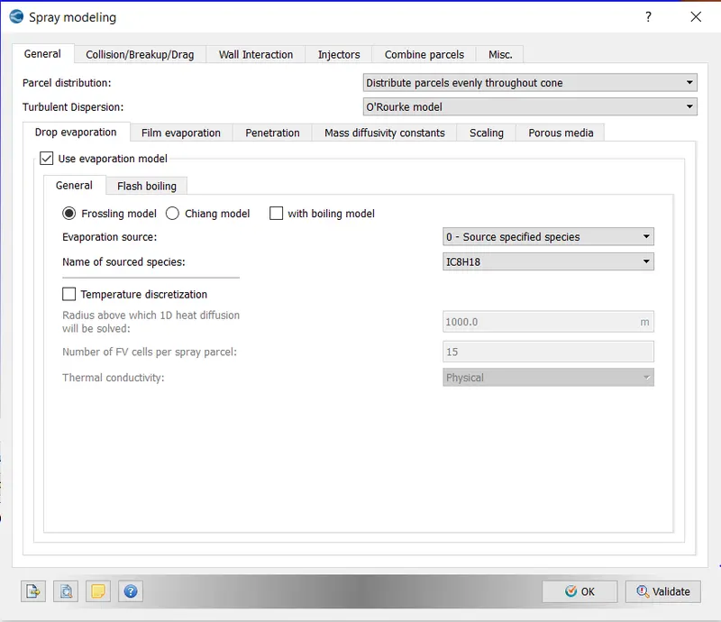
Drop evaporation:

Parcel distribution: Distribute parcels evenly throughout the cone.

Turbulent dispersion: O’Rourke model

Evaporation modelling: Frossling model

Evaporation source: Source specified species

Sources species: Iso-octane (IC8H18)

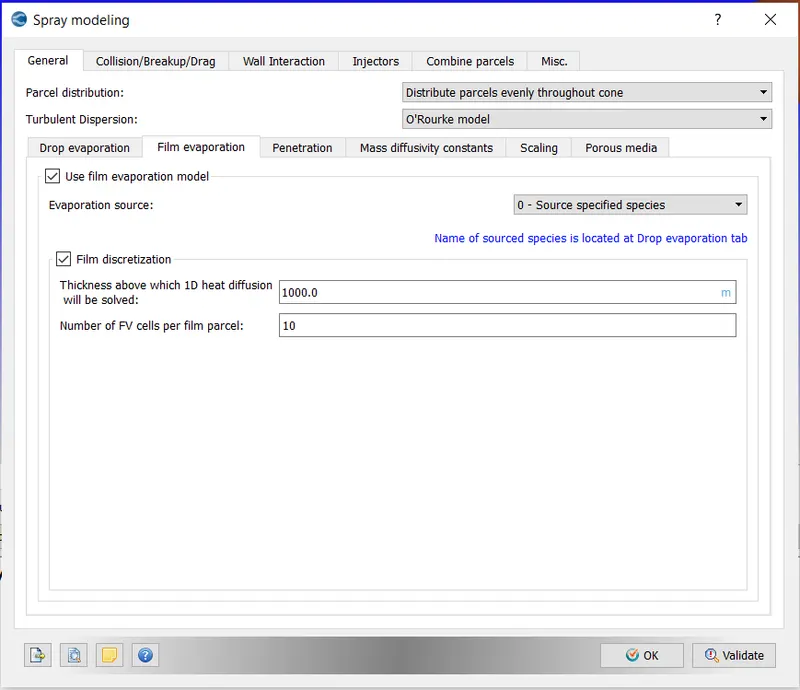
Temperature discretization is not required since it will take more computational time.

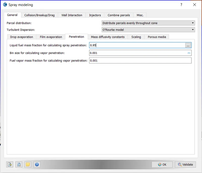
Penetration:

Liquid fuel mass fraction for LPL: 0.95

Bin-size: 0.001

Fuel vapour mass fraction for VPL: 0.001

Collision/Breakup/Drag:

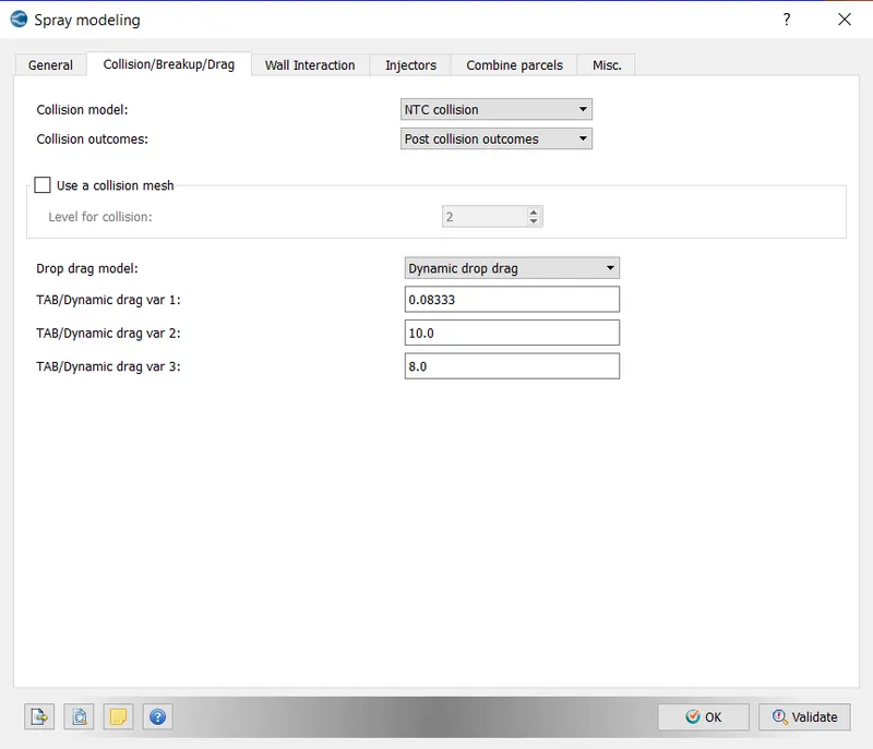
Collision model: NTC collision

Collision outcomes: Post-collision outcomes

Tick use collision mesh for realistic animation.

Drop drag model: dynamic drag model.

Wall-interaction:

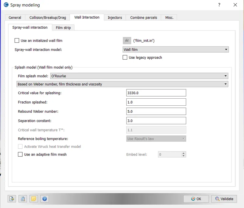
Spray-wall interaction:

Model: Wall film

Formation of film on the surface of the liner on which splash of fuel parcel occurs.

Splash model:

Model: O’Rourke

Based on weber number, film thickness, and viscosity.

Weber number: It is a ratio of inertial force (force responsible for momentum) to that of surface tension force (Stronger cohesive force between molecules).

Injector:

Add injector and click edit.

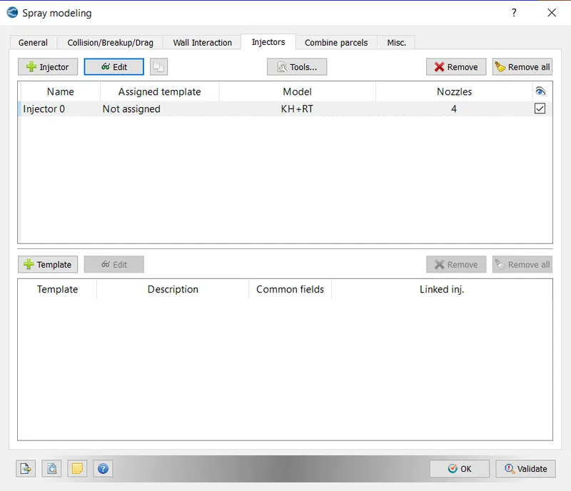
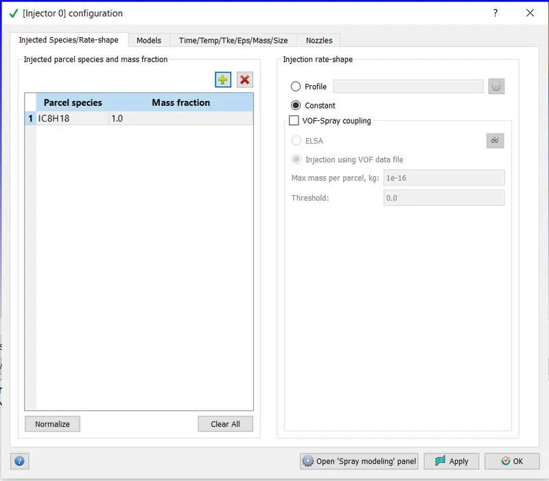
Injected species:

Iso-octane, and we can add a profile to specify when the fuel injection should start and end.

Models:

Kelvin Helmholtz model (KH)

Rayleigh Taylor model (RT)

Discharge coefficient model.

We have a set of recommended values for some fuels we can use for setting the above models for injection modelling

Time/Temp/Tke/Eps/Mass/size:

Injection type: cyclic

Cyclic period: 720 degrees (for one cycle)

Start of injection: -480 deg (before the suction stroke)

Injection duration: 191.2 deg (We should inject fuel for a specified time we can convert it in terms of deg based on rpm of our engine).

Total injected fuel mass (kg):

Given,

RPM = 3000

Fuel flow rate = 7.5*e­­­­­­­^-04

Time taken per cycle:

t = 2*60/N (Since for each cycle there is 2 complete rotation)

t = 2*60/3000

t = 0.04s

Time taken for 1cycle (720 deg) is 0.04s then time taken per deg = 0.04/720

= 5.55*e^-05

Fuel mass per cycle = fuel flow rate (kg/s) * time taken per cycle

= 3*e^-05

So the value for Total injected mass (kg) = 3*e^-05

Nozzles:

Nozzle location and orientation: Cartesian

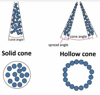
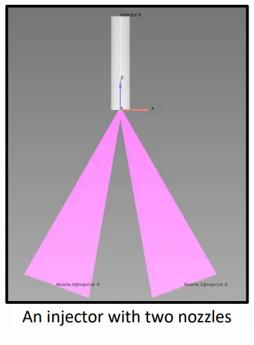
We should specify 4 nozzles for the same injector for injection of the spray:

Nozzle diameter: 0.00025m

Spray cone angle: 10deg

Location and orientation for 4 nozzles:

Nozzle 0

• center 0.0823357 0.00100001 0.07019
• Align Vector -0.732501 0.210489 -0.647408

Nozzle 1

• center 0.0823357 -0.00099999 0.07019
• Align Vector -0.732501 -0.210489 -0.647408

Nozzle 2

• center 0.0823357 -0.0004 0.07019
• Align Vector -0.5 -0.2 -0.647408

Nozzle 3

• center 0.0823357 0.0003 0.07019
• Align Vector -0.5 0.2 -0.647408

Injection spray type solid cone spray in case of hollow cone spray the LES model should be selected.

Combustion modelling:

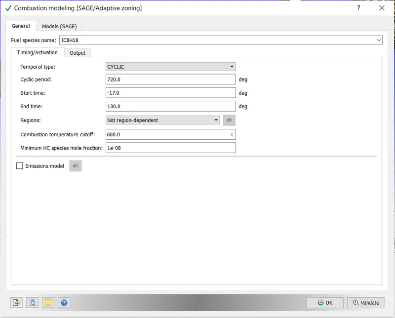
General:

Fuel species: IC8H18

Temporal type: Cyclic

Cyclic period: 720 deg

Combustion modelling should be ready before spark ignition and should end when the exhaust port opens.

Start time: -17 deg

End time: 130 deg

Acceleration parameters:

Combustion temperature cut-off: 600K

Minimum HC species: 1*e^-08

Models:

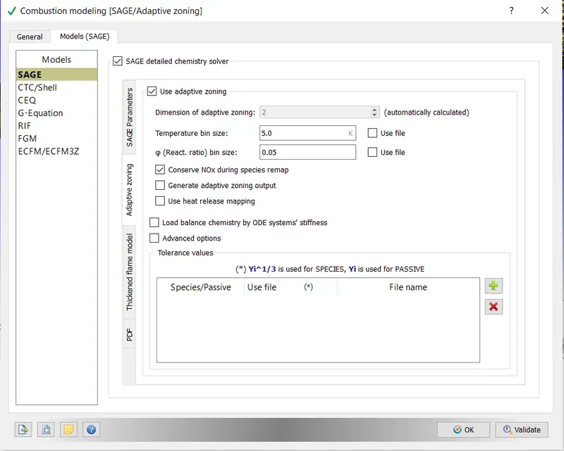
SAGE model

Temperature bin size: 5K

Equivalence ratio bin size: 0.05

If the difference in temperature and equivalence ratio of cells is less than specified, the cells are grouped into one cell.

Source/sink modelling:

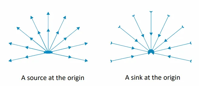
In this we should specify the source for ignition(spark) its temperature, amount of energy, start and end time.

The total deg for which we should initiate Spark is 10deg and spark must be triggered during the start of combustion in our simulation the combustion stroke is between -17 to 130 deg, The time duration for spark is very small (µs) and a large amount of energy is been generated.

The best spark timing is typically 15-35 degrees before TDC (top dead center) of power stroke depending on the engine speed. Best power is achieved when ignition timing is set to fire the spark ahead of time to reach that peak pressure at about 2 degrees after TDC.

Energy: 0.04 joules for -15.0 to -14.5 deg, and 0.02 joules for -15.0 to -5 deg.

Grid Control:

Base grid: 0.008m

Adaptive mesh refinement:

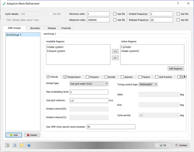
Adaptive mesh refinement must be applied to Cylinder and intake systems, major changes in velocity and temperature occur in the cylinder during the combustion process so cells must be refined to capture detailed chemical kinetics.

Temperature:

Embedding level: 3

Sub-grid criterion: 2.5K

For temperature, we should specify the time in which AMR should be active to reduce computational time.

Timing control type: Cyclic

AMR start: -17 deg

AMR end: 131 deg

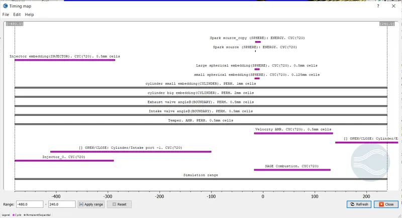
The above range is for expansion/power stroke. We can always compare time map select values for any process.

Velocity:

Embedding level: 3

Sub-grid criterion: 1m/s

Timing control type: permanent

Fixed embedding:

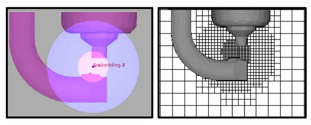
Embedding must be provided surrounding to spark plug since there is a gradual increase in temperature during spark which cannot be accounted for by AMR because of larger cells, these cells surrounding the spark plug should be refined before spark generation to calculate accurate results.

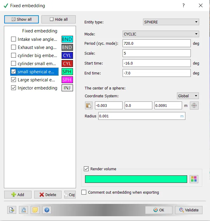
Two spherical embeddings must be provided surrounding the spark one large and one small.

Spark plug small embedding:

Radius: 0.001m

Scale: 5

Start time: -16 ( 1 deg before spark start time)

End time: -7( 2 deg ahead of the spark end time)

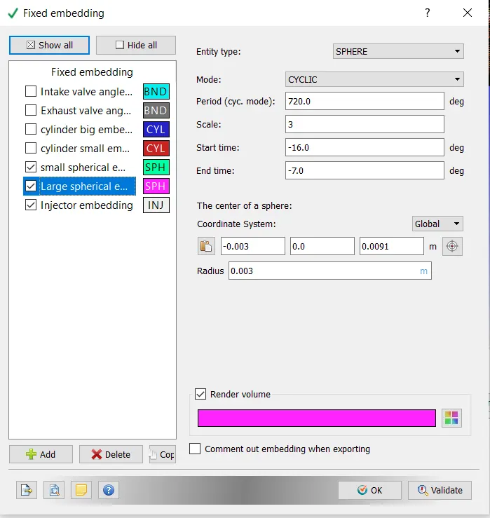
Spark plug large embedding:

Radius: 0.003m

Scale: 3

Start time: -16 (1 deg before spark start time)

End time: -7 (2 deg ahead of the spark end time)

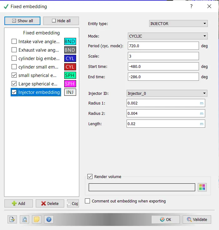
Injector embedding:

To capture the velocity parcel data during injection of fuel.

Entity type: Injector

Mode: cyclic

Scale: 3

Radius 1: 0.002

Radius 2: 0.004

Length: 0.02

Time map for all processes:

Output/Post-processing:

We should include the species mass fraction and passive as our output.

RESULTS:

Plots:

Pressure volume diagram:

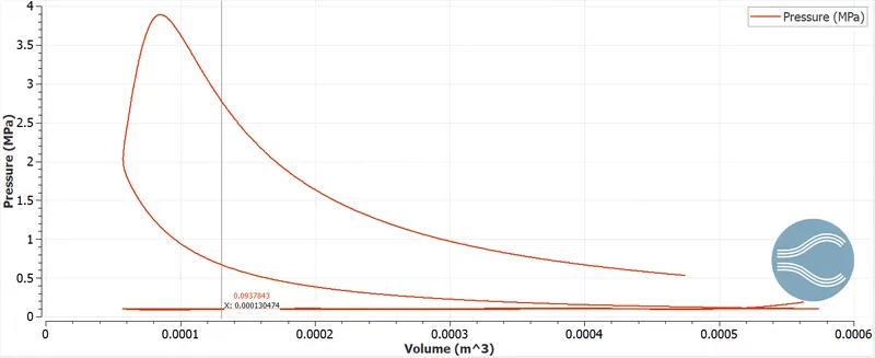
This plot can be used to visualize the four strokes of the 4-Stroke IC engine and the area under this plot is work done.

Mean temperature:

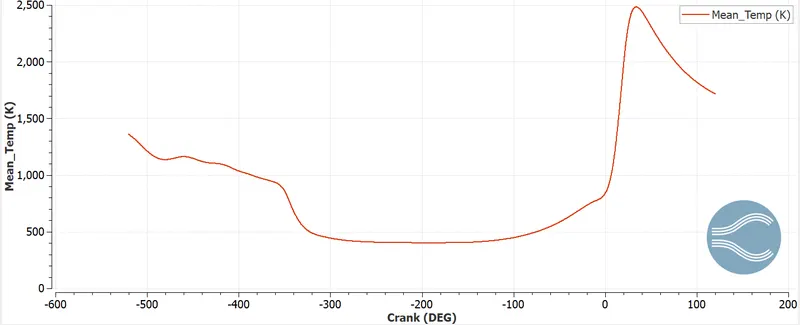
The maximum temperature from the above plot can be used to calculate the heat transfer at the wall where this can be used as a boundary condition (Dirichlet boundary condition).

Volume:

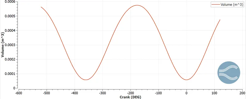
Can be used to calculate the compression ratio of the SI engine.

Gamma:

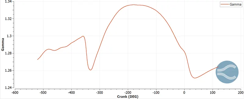
We use gamma value in the calculation of efficiency where we should include the changes in gamma value rather than taking a constant value.

Integrated heat release rate(HRR):

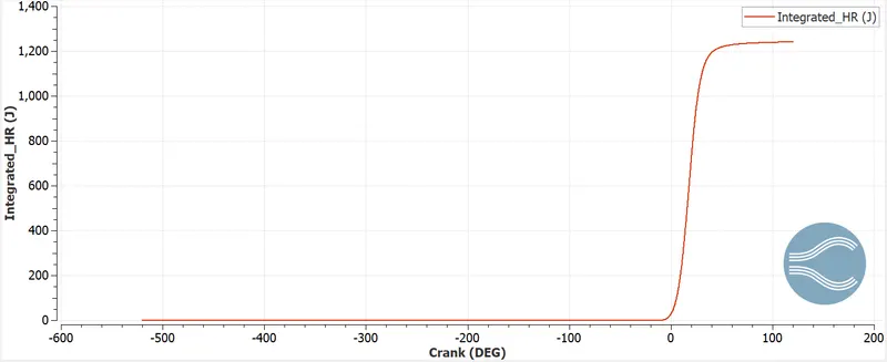
The peak value of the heat release rate can be used to calculate combustion efficiency.

Species mass:

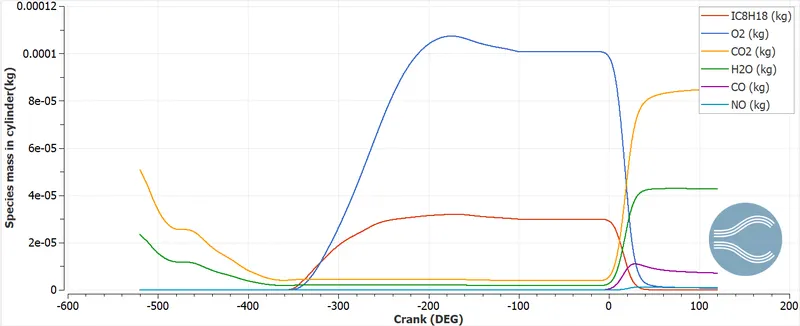
How the reactants and product mass change in the cylinder for the whole cycle, and also provide the mass of NOx and CO to find emissions caused.

Liquid drops:

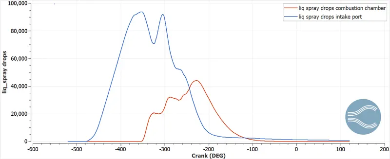
The plot shows how the quantity of parcels changes from intake to exhaust and we can generally find the trapped fuel mass.

Fuel mass(IC8H18):

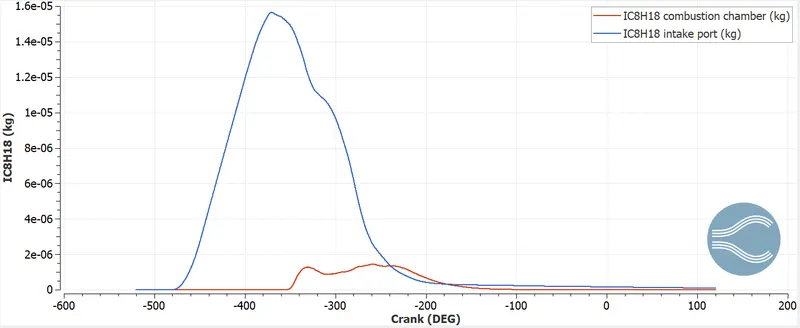
The fuel mass in intake plot and cylinder due to burning of fuel in combustion process the mass of fuel decreases.

Cell count:

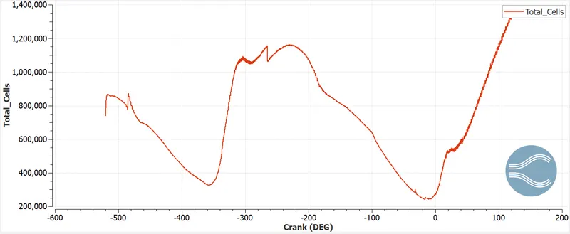
The cell count changes during a cycle because of adaptive mesh refinement.

Engine Performance calculation:

1. What is the compression ratio of this engine?

Compression ratio:

It is the ratio between the total volume of a cylinder to the clearance volume.

R_c = (V_s + V_c) / V_c

R_c = 10.05:1

V_s = Swept volume

V_c = Clearance volume

2. Use the engine performance calculator, to determine the power and torque for this engine?

Values extracted from the simulation:

Gross indicated work done = 468.646 Nm

Indicated mean effective pressure(IMEP) = 896428 pa or N/m²

Heat release rate (HRR) = 1241 J(From HRR plot)

RPM = 3000

Fuel flow rate = 7.5*10^-04

Time taken per 720 deg = 0.04 s

Duration from start of power stroke to end of exhaust stroke in deg = 240.199 deg

Time taken by 240.199 deg is = (240.199 * 0.04) / 720

= 0.0133 s

Power = Work done(Nm) / Time taken

= 468.646 / 0.013

= 35236 Nm/s

= 35236 Nm/s * (1 KW/ 1000 Nm/s)

= 35.236 KW

The power we got here is indicated power since power was generated in the cylinder due to the burning of fuel and is acting on the piston.

To calculate torque we need brake power. Brake power is power at crankshaft which will always less than the indicated power but in our case, there is no frictional loss, so the brake power is equal to indicated power.

FP = IP – BP

0 = IP – BP

IP = BP

Brake power formula is given as(BP) = (2*π*N*T) /(60000)

T = (35.236 *60000)/( 2*3.14*3000)

T = 112.21 Nm

Efficiencies:

Brake thermal efficiency (η_bth) :

η_bth = BP / (m_f * C_v)

= (35236 J/s) / (7.5*10^-04 (Kg/s) * 4.77*10⁷ (J/kg)

= 0.98 *100 = 98%

(η_bth) = (η_Ith)

3. Calculate the combustion efficiency of this engine?

Combustion efficiency (η_c):

η_c = Heat release rate /(m_f * C_v)

= 1241(J) / (3*10^-5(Kg) *4.77*10⁷(J/kg))

= 0.865*100

= 86.5%

Mechanical efficiency (η_mech):

η_mech mechanical efficiency is 100% for our engine since there are no frictional losses due to mechanical components but in general, there is always a frictional loss.

Specific fuel consumption (SFC):

Ratio of mass of fuel used to the indicated or brake power generated.

SFC = m_f (Kg/hr) / (BP or IP(KW))

= 7.5*10^-4*3600 / (35.236)

= 0.076 kg/kWhr

= 76 g/kWhr

• Since the power, the engine developing is less the specific fuel consumption is less.
• If the specific fuel consumption is low even for higher horsepower then the engine efficiency is greater.

4. What is the significance of ca10, ca50, and ca90?

CAD10: crank angle at which 10% of the fuel is burnt.

CAD50: crank angle at which 50% of the fuel is burnt.

CAD90: crank angle at which 90% of the fuel is burnt.

The significance of CAD10 to determine the time taken for ignition(ignition delay). If the required temperature is high( Since the ignition delay is mainly dependent on temperature) the ignition will take place faster. The value for CAD10 of the Pfi engine is 6.83727 deg.

The significance of CAD50 is to estimate how fast the flame is traveling, the faster the flame front is faster the fuel is burnt and the greater the power. The value for CAD50 of the Pfi engine is 18.46 deg.

The significance of CAD90 is to estimate the time take for the combustion process since almost all the fuel is burnt at this point. The value for CAD90 of the Pfi engine is 31.401 deg.

5. Why do we need a wall heat transfer model? Why can't we predict the wall temperature from the CFD simulation?

• Heat transfer in engines affects engine efficiency and emission.
• An increase of heat transfer to the combustion chamber walls will lower the in-cylinder pressure and the average gas
  temperature and thus reduces the work per cycle transferred to the piston.
• Thus, the magnitude of engine heat transfer is strongly dependent on engine efficiency.
• The changes in the gas temperature due to heat loss through the combustion chambers also have an impact on the pollutant emission formation. A higher in-cylinder temperature promotes the NOx emissions and the lower in-cylinder temperature
  causes the particulates during the exhaust.
• Since the engine heat transfer is important, accurate predicted engine heat transfer results are needed.
• To obtain accurate values of heat flux, a multi-dimensional model for core regions and one-dimensional heat transfer near walls are necessary. Since the mechanism of wall layers is similar to the physics in the boundary layers, the predicted heat fluxes were solved by using thermal boundary layer assumptions.

The wall heat transfer model is used to calculate the gas-phase heat transfer near-wall regions. The analysis of the formulations of this model is initiated from the one-dimensional energy equation across the boundary layer which is described below in the equation.

where ρ and T are the fluid density and temperature near walls respectively, Cp is the specific heat at constant pressure, P is pressure, v is the fluid velocity, k is laminar thermal conductivity, kt is turbulent thermal conductivity and Q is volumetric heat release rate.

Several assumptions are introduced in the derivation of the model, including the following:

(1) Fluid velocity near walls is parallel to the wall, and only the temperature and density gradients normal to the wall are considered.

(2) The gas is assumed to be ideal.

(3) The pressure is uniform in space

(4) Viscous dissipation is neglected.

(5) Radiation heat transfer is not included.

Based on these previous assumptions, the wall heat flux in the near-wall regions is computed by equation.

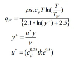
where qw is heat flux on the wall, u* is friction velocity, y+ is the dimensionless distance, Tw is the wall temperature, ν is the kinematic viscosity, tke is turbulent kinetic energy and Cµ is equal to 0.09.

The heat transfer for the wall will not be calculated by CFD simulation if we don't provide the wall parameters (i.e. wall material, thickness, thermal conductivity, etc.), in our simulation, we have only solved for core region for gas inside the combustion chamber, to solve for wall region and core region together we can use conjugate heat transfer model and specify the interface boundary between solid and gas and wall parameters.

Video link:

https://drive.google.com/file/d/1CTWe6X8SUMAAImxqPMh4IzKu_yh-3sdn/view?usp=sharing

Conclusion:

Compression ratio (R_c)= 10.05:1

Specific fuel consumption (SFC) = 76 g/kWhr

Gross indicated work done (W) = 468.646 Nm

Heat release rate (HRR) = 1241 J(From HRR plot)

RPM = 3000

Time taken per 720 deg = 0.04 s

η_mech (Mechanical efficiency)= 100%

η_c (Combustion efficiency)= 86.5%

Thermal efficiency (η_bth) = (η_Ith) = 98%

Torque (T) = 112.21 Nm

Power (P) = 35.236 KW

The NOx emission is less which is a good part of this engine and the in-cylinder temperature is also higher due to which the NOx emission is less.

But the higher temperature causes more amount of CO(Carbon monoxide) emissions.

But overall the higher temperature is suitable since it will burn all the fuel which will result in minimum emissions.