Week 10: Modeling and Simulation of flow around an Ahmed Body

MODELING AND SIMULATION OF FLOW AROUND AN AHMED BODY

AIM: The aim of this project is to model and simulate the flow over Ahmed body in converge.

OBJECTIVE:

• Create the CAD model using your any CAD package (50 points)
• Setup a Coarse CFD simulation (300 points)
  • Setup the virtual wind tunnel as shown in the video
  • Apply the right boundary conditions and solver settings (50 points)
  • Use a coarse mesh to demonstrate that your setup runs successfully (150 points).
    • You need to show an animation of the velocity distribution on a cutplane. This cutplane should cut the ahmed body model in two symmetric pieces.
    • You need to show an animation of the pressure distribution on a cutplane. This cutplane should cut the ahmed body model in two symmetric pieces.
    • Post process the coarse mesh results and extract the x component of velocity along a line(Here, I am assuming that the normal of the intake boundary is along the +x direction)
    • The line should be perpendicular to the ground plane.
  • Enable wall-averaged outputs to measure the drag and lift forces (100 points)
    
    • Calculate the steady state drag force value and explain your calculation procedure.
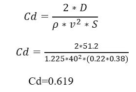
    • Calculate the drag co-efficient using paraview and explain your calculation process in detail

THEORY:

The Ahmed body is a generic car body (a simplified vehicle model). The airflow around the Ahmed body captures the essential flow features around an automobile and was first defined and characterized in the experimental work of Ahmed. Although it has a very simple shape, the Ahmed body allows us to capture characteristic features that are relevant to bodies in the automobile industry. This model is also used to describe the turbulent flow field around a car-like geometry. Once the numerical model is validated, it is used to design new models of the car.Ahmed body is simplified car model created by Ahmed et in the 1980s to investigate the behaviour of newly developed turbulence models for complex geometry cases. The Ahmed body is made up of around front part, a movable slant plane placed in the rear of the body to study the separation phenomena at different angles, and a rectangular box, which connects the front and rear slant plane as shown. Ahmed body is a simplified model of a car body, but it demonstrates all the flow features involved in an actual case of a moving car. Current vehicle development needs a strong background in aerodynamics to improve flow control by means of active or passive control devices. The complexity involved in the automobile design especially due to the great number of accessories and devices that form its geometry makes the validation tasks unaffordable. The Ahmed model is a simple geometric body that retains the main flow features, especially the vortex wake flow where most part of the drag is
concentrated and it is a good candidate to be used as a benchmark test.The Ahmed body represents a simplified, ground vehicle geometry of a bluff body type. Its shape is simple enough to allow for accurate flow simulation but retains some important practical features relevant to automobile bodies. Selection of the configuration of this body is governed by the requirement that it should generate the essential features of a real vehicle flow field except for the flow fields that occur due to rotating wheels, engine and passenger compartment, rough underside and surface projections. The model chosen would generate strong 3-D flows in front, relatively uniform flow in the middle and a large structured wake at the rear.

Reason for negative pressure in the wake region:

The path lines showing the exact circular motion or vorticity generation just at the rear end of the car. The separation takes two regions of distribution. One at the upper part of the rear and the other at the lower part of the rear end.

The path lines show about the nature of the fluid interaction with the rear end of the Ahmed body which here shows that the fluid just after leaving the contact from the slope still possess the momentum in it and the fluid particles near to the surface almost show the no-slip region which means the very least possible velocity of the fluid particles is in contact with the slope and base of the rear part. Thus the fluid particles away from the rear region having the higher pressure beside the wake region try to approach from the higher pressure region to the lower pressure region thus creating a circularity exactly in the wake region created.The body penetrating the fluid creates a region of emptiness just beside its end due to the nature of the geometry of the body here which can be seen least in case of a perfectly streamlined shaped body. This emptiness created is a low-pressure region towards which the fluid column exactly behind the wake region which of atmospheric pressure tries to fill the space thus dragging the fluid column with it thus creating the region of vorticity. This also results in the huge pressure gradient in the region exactly rear of the body creating the –ve pressure at the end. Also, this is the layman’s reason why there is negative gauge pressure in the wake region.

SIMULATION AND SOLUTION:

GEOMETRY

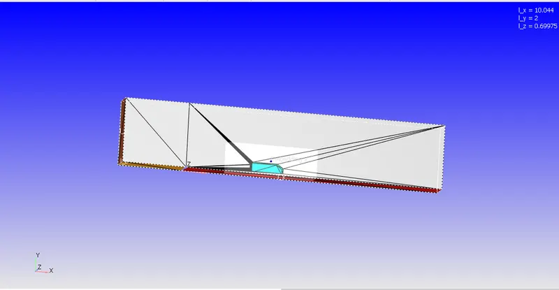
Using the following standard Ahmed Body geometry dimension, the geometry was created using CAD software and then imported in Converge.

The wind tunnel is created in such a way that the front of the body is placed at a distance of 2 car lengths (2L) from the flow inlet. To reduce the computational cost, a symmetry plane is introduced to model half of the model.

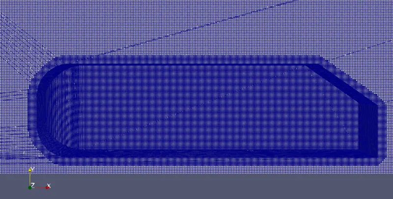
The flow for this model is turbulent, which is based on the Reynolds number determined by the body length and inlet velocity. The simulation solves for the turbulent kinetic energy in addition to the velocity field. For this simulation, we need a larger mesh size than what is usually common to resolve the turbulent flow. More specifically, we use a finer mesh downstream of the model to capture the wake zone.

The flow for this model is turbulent, which is based on the Reynolds number determined by the body length and inlet velocity. The simulation solves for the turbulent kinetic energy and dissipation in addition to the velocity and pressure fields.

Setup

Application Type	Time-based
MATERIALS:
1. Gas simulation	Standard
2. Global Transport Parameters	Standard
4. Species	O2 and N2
SOLUTION PARAMETERS
1. Run Parameters	Transient >Full hydrodynamic>Compressible
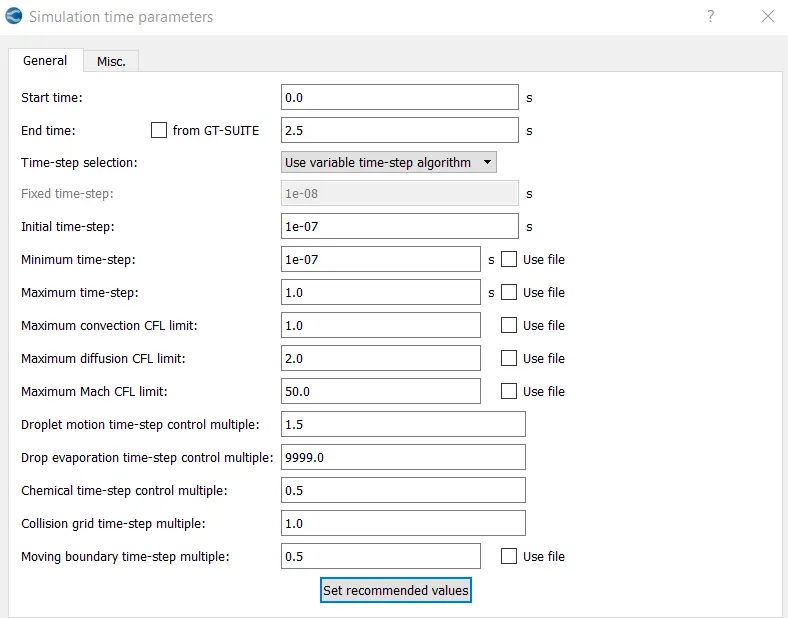
2. Simulation time parameters
3. Solver parameters	Navis-stokes solver scheme: PICO Navis-stokes solver type: density-based
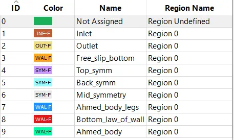
BOUNDARY CONDITIONS
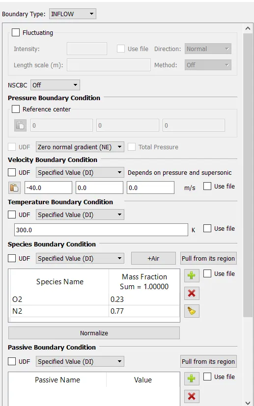
1. Inlet
2. Outlet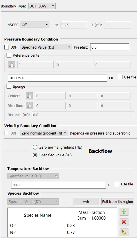
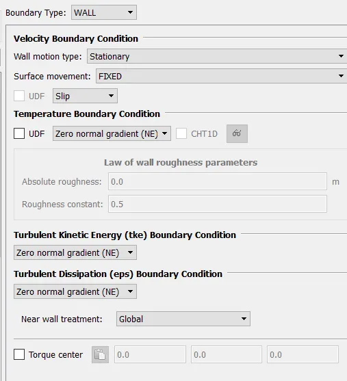
3. free_slip_bottom
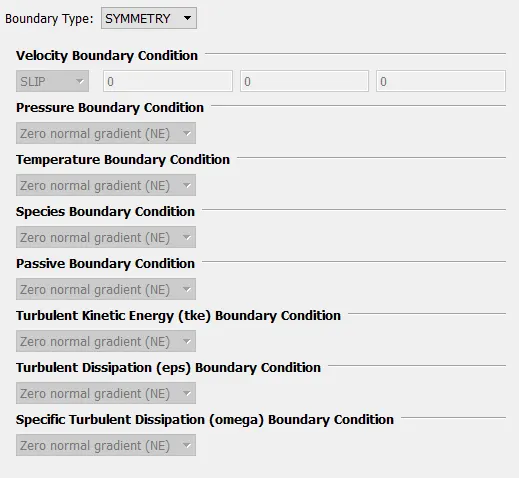
4. Top_symmetry
5. Back_symmetry
6.Mid_symmetry
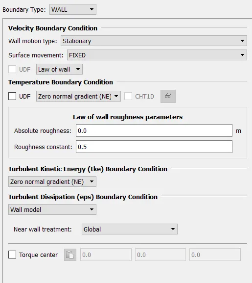
7. Ahmed body legs
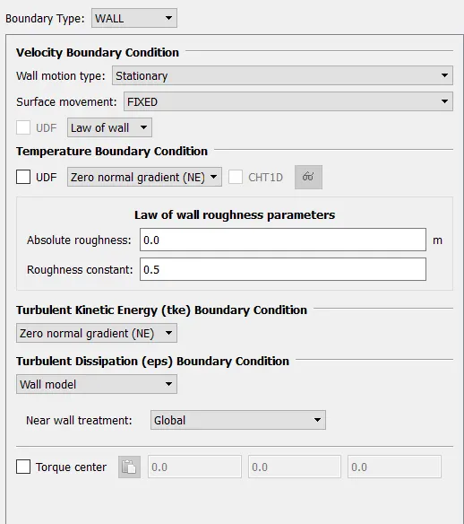
8. Bottom law of wall
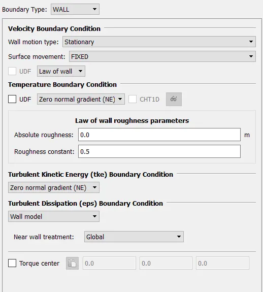
9. Ahemd body
INITIAL CONDITIONS AND EVENTS
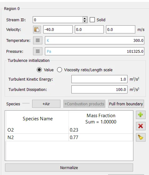
1. Regions and initialization
PHYSICAL MODELS
1 Turbulence modeling	RNG-k-epsilon
GRID CONTROL
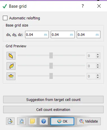
1. Base mesh
2. Fixed meshing
OUTPUT/POST-PROCESSING
1. Post variable selection	Standard
2. Output files:

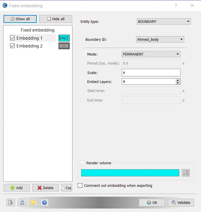
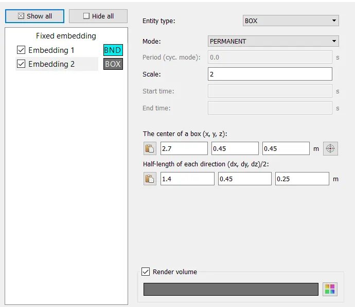
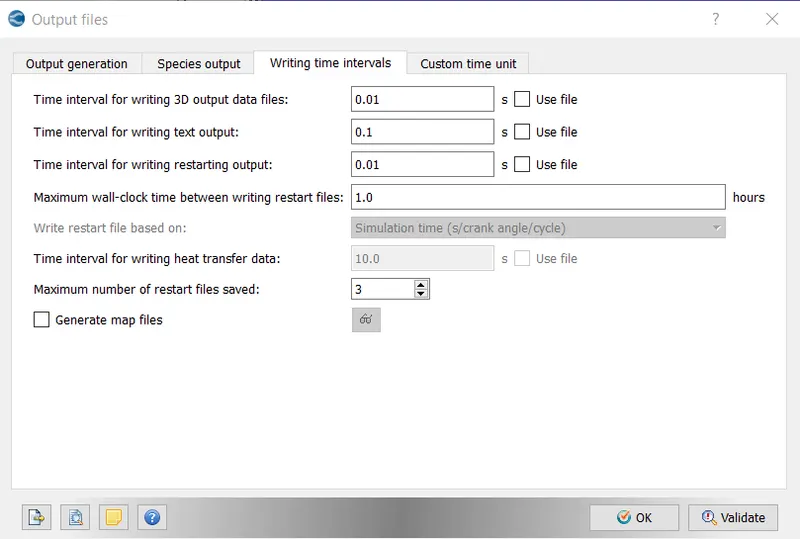
Then Export the Files

Then continuing the setup in Cygwin :

• leading to the folder where the exported files are saved
• Then using mpiexec.exe -n 2 converge.exe restricted to simulate the setup
• After the output is generated, we lead the Cygwin to the output folder, and by copying the post_convert folder and
• Using mpiexec.exe -n 2 post_convert.exe and converting these files for processable output in ParaView.

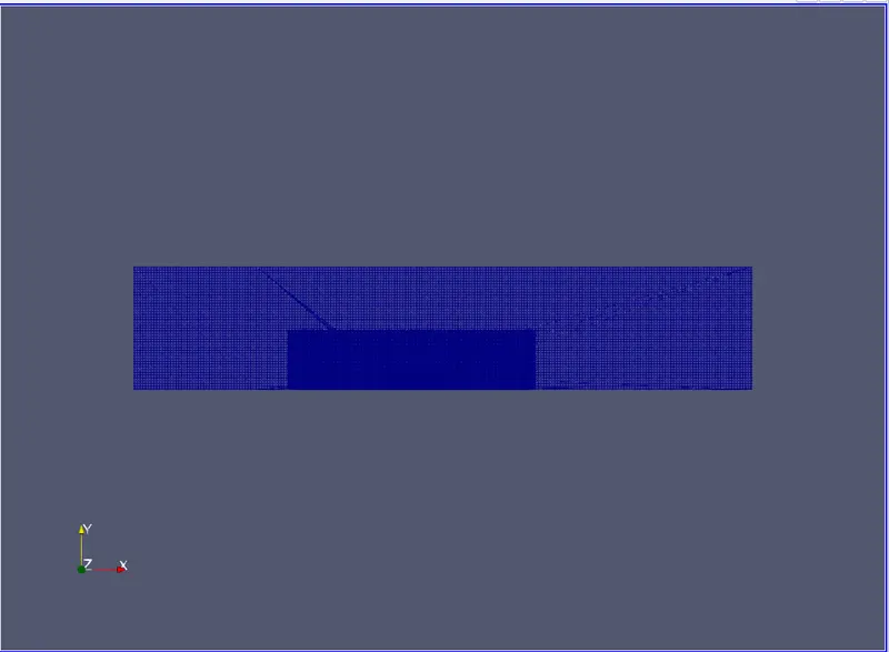
MESH:

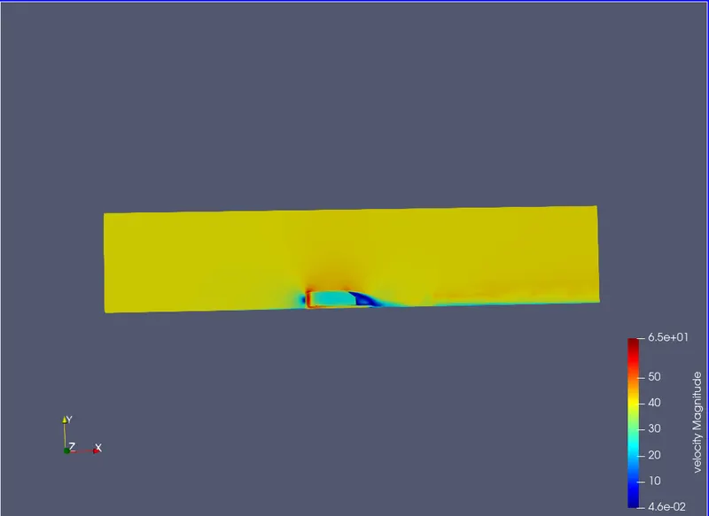
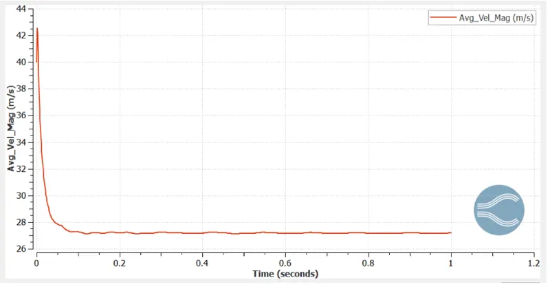
VELOCITY COUNTER

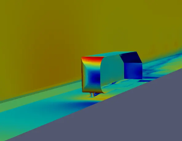
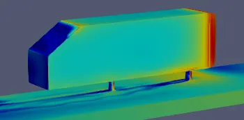
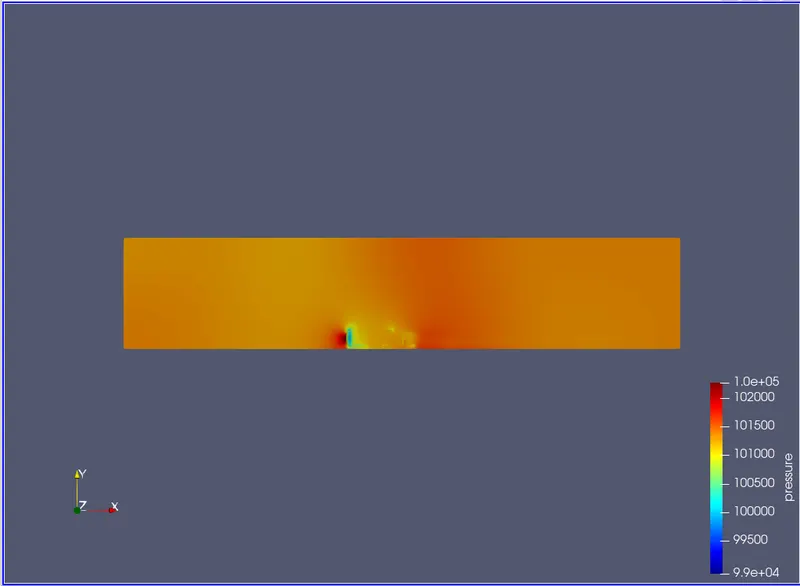
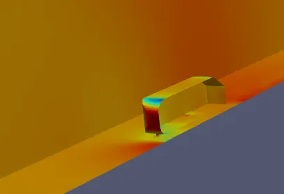
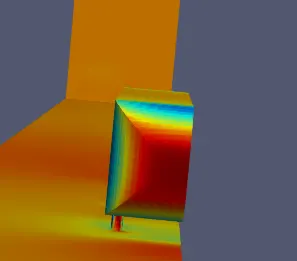
PRESSURE COUNTER

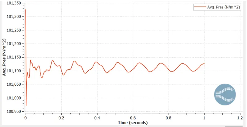
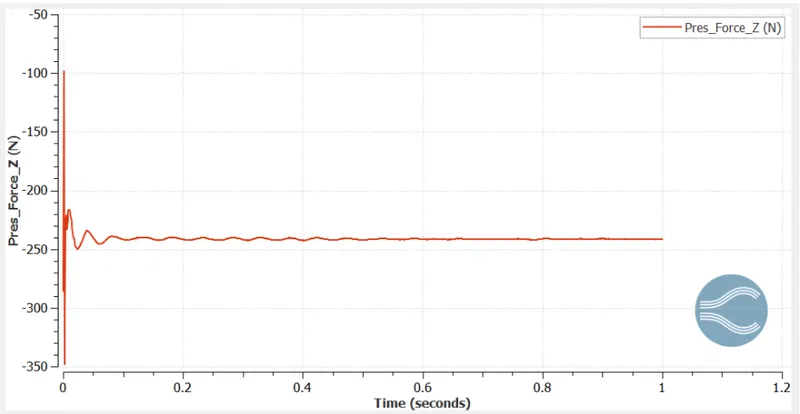
L=-240N

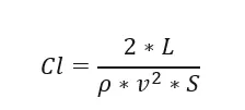
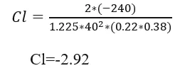
Coefficient of lift,

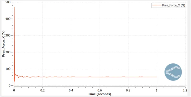
D=51.2N

Experimental vs Simulation Data:

The following plots are made in excel sheets using the simulation and experimental data. In order to analysis the obtained data with experimental results we need to plot the line probes for different locations in the body w.r.t the velocity of the flow around it. This helps us to know the velocity at different locations on or above the body.

The charts represent the velocity values at various points in the wind tunnel

From the above graphs we can see that deviation that we have is acceptable and the results are good to be trusted.

CONCLUSION:

• From the graphs, we can see that the probes at the negative location are matching well with the experimental data compared to the probes on the positive side.
• On the positive side, we can see that the error percentage in the graphs is greater than 5%. This is because of the grid size. We can reduce the grid size or simulate only one symmetric half with reduced grid size.
• The error on the positive side is greater because of the Drag produced on the rear side of the body. The rear side is positive from origin.
• To capture this wake region correctly a smaller grid size and greater computational power are required.
• From the Velocity contour, it is observed that after passing through the geometry there is a region where recirculation happens this region is called as wake region. Due to this low pressure, the air at the front tries to come back which increases the drag.
• The air after exiting the cylindrical pillars forms vortices. These vortices can be observed from the top view.
• It is also observed that the lift obtained is negative which means that it is downward force. This force helps racing cars to stay on the ground. But for a low-efficiency vehicle such as a truck, this force is not desirable. Hence the shape of the truck/trailer will be optimized to reduce the negative lift.