Week 10: Modeling and Simulation of flow around an Ahmed Body
Week 10: Modelling and Simulation of flow around an Ahmed Body
Aim:
- To create the CAD model using your any CAD package.
- To setup a Coarse CFD simulation.
- To setup the virtual wind tunnel as shown in the video.
- To apply the right boundary conditions and solver settings.
- To use a coarse mesh to demonstrate that your setup runs successfully.
- To calculate the steady state drag force value and explain your calculation procedure.
- To calculate the drag co-efficient using paraview and explain your calculation process in detail.
Introduction:
Ahmed Body:
The automobile industry is evolving as well as flourishing in the entire world day by day. This development has massive impact on air pollution and climate change in our planet. Developing aerodynamically efficacious vehicle will reduce the fuel consumption and it is the major way to mitigate air pollution and climate change crisis in the world.
The Ahmed body is a generic car body (a simplified vehicle model). The airflow around the Ahmed body captures the essential flow features around an automobile and was first defined and characterized in the experimental work of Ahmed. Although it has a very simple shape, the Ahmed body allows us to capture characteristic features that are relevant to bodies in the automobile industry. This model is also used to describe the turbulent flow field around a car-like geometry. Once the numerical model is validated, it is used to design new models of the car.
Ahmed body is simplified car model created by Ahmed et in the 1980s to investigate the behavior of newly developed turbulence models for complex geometry cases. The Ahmed body is made up of around front part, a movable slant plane placed in the rear of the body to study the separation phenomena at different angles, and a rectangular box, which connects the front and rear slant plane as shown. Ahmed body is a simplified model of a car body, but it demonstrates all the flow features involved in an actual case of a moving car. Current vehicle development needs a strong background in aerodynamics to improve flow control by means of active or passive control devices. The complexity involved in the automobile design especially due to the great number of accessories and devices that form its geometry makes the validation tasks unaffordable. The Ahmed model is a simple geometric body that retains the main flow features, especially the vortex wake flow where most part of the drag is concentrated and it is a good candidate to be used as a benchmark test.
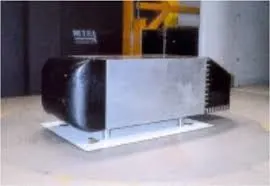
The Ahmed body represents a simplified, ground vehicle geometry of a bluff body type. Its shape is simple enough to allow for accurate flow simulation but retains some important practical features relevant to automobile bodies. Selection of the configuration of this body is governed by the requirement that it should generate the essential features of a real vehicle flow field except for the flow fields that occur due to rotating wheels, engine and passenger compartment, rough underside and surface projections. The model chosen would generate strong 3-D flows in front relatively uniform flow in the middle and a large structured wake at the rear.
Drag:
It is the common force that a body meets some resistance when it is forced to move through a fluid. We could notice that we feel difficult to walk in water because of the much greater resistance it offers to motion compared to air. A fluid may exert forces and moments on a body in and about various directions. The force a flowing fluid exerts on a body in the flow direction is called drag. The drag forces can be measured directly by simply attaching the body subjected to fluid flow to a calibrated spring and measuring the displacement in the flow direction experimentally. The most researches have been centred around the reduction of drag. Reduction of drag is closely associated with the reduction of fuel consumption in automobiles. But in certain cases, drag produces a beneficial effect and we try to maximize it.
Drag force is proportional to the velocity for low-speed flow and the squared velocity for high-speed flow, where the distinction between low and high speed is measured by the Reynolds number. Drag forces always tend to decrease fluid velocity relative to the solid object in the fluid's path.
The drag depends on the density of the fluid, the upstream velocity, size, shape of the body. The drag co-efficient is calculated by using the following formula.
`F_D=1/2 *rho*v^2*C_D*A`
where
`F_D` is the drag force
`rho` is the density of the fluid
`v` is the velocity of the fluid
`A` is the cross sectional area
`C_D` is the drag co-efficient.
Lift:
A fluid flowing around an object exerts a force on it. Lift is the component of this force that is perpendicular to the oncoming flow direction. It contrasts with the drag force, which is the component of the force parallel to the flow direction. Lift conventionally acts in an upward direction in order to counter the force of gravity, but it can act in any direction at right angles to the flow.
The lift co-efficient is calculated by using the following formula.
`F_L=1/2*rho*v^2*C_L*A`
where
`F_L` is the lift force
`rho` is the density of the fluid
`v` is the velocity of the fluid
`A` is the cross sectional area
`C_L` is the lift co-efficient.
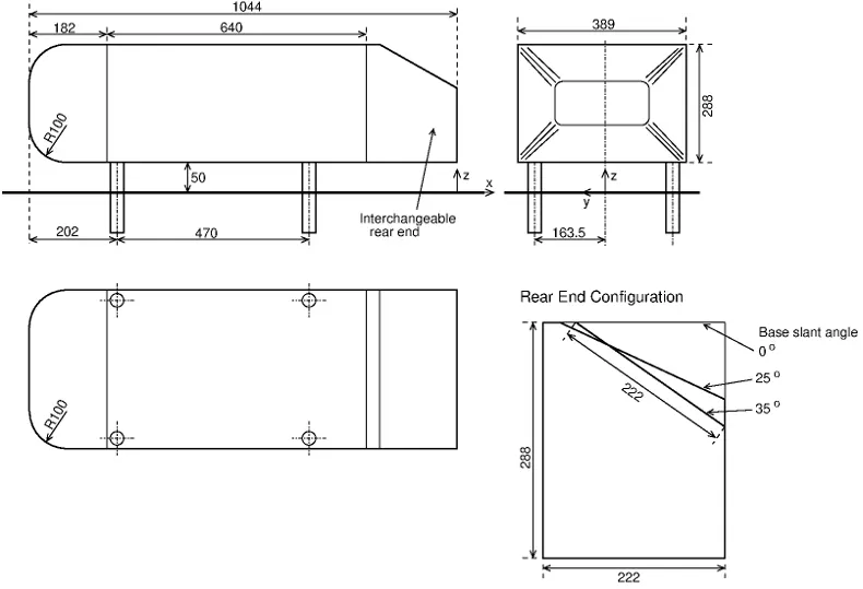
Ahmed Body Geometry:
Modelling:
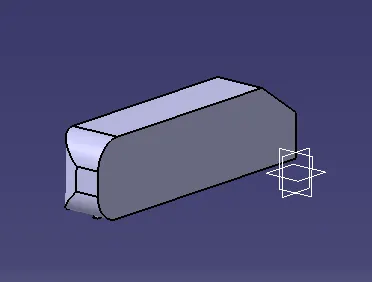
By using the dimensions mentioned above, the Ahmed body model was designed using CATIA V5R20 software. In order to make the model simpler, as the Ahmed body was considered to be symmetrical, only the half of its body was designed using the designing software.
Slant angle of 35º used at the rear end since experimental data is available for this angle. All other dimensions of the Ahmed body are made exactly equal to the original geometry. Import the file of the designed Ahmed body in STL extension which can be imported in Converge.
Geometry Setup:
Once the STL file is imported in Converge, the model is scaled down to the scale factor of 0.001.
The virtual wind tunnel is setup by the following calculations.
Distance Calculation for the growth of Boundary Layer:
The boundary layer of thickness 30mm should be developed at a distance of 400mm in front of the Ahmed Body.
The formula for approximating the boundary layer thickness over a flat plate is given by,
`δ=(0.382*x)/(Re)^(1/5)`
where,
`δ`= Boundary Layer Thickness = 0.03m
Re is the Reynolds number = 768,000.
X is the distance from the boundary layer.
Calculation:
`X=(δ.(Re)^(1/5))/0.382`
`X=(0.03*(768000)^(1/5))/0.382`
X=1.1806
Virtual Wind Tunnel Dimension:
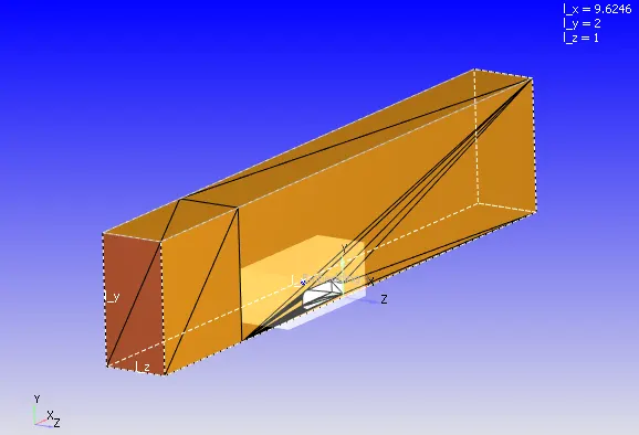
X = 9.6246 m
Y = 2 m
Z = 1 m
In x-axis 2 m for slip region, 1.18 m + 0.4 m for boundary layer formation, 1.044 for the length of the Ahmed Body, 5 m at the back side of the Ahmed body.
X = 2.0 + 1.18 + 0.4 + 1.044 + 5
X = 9.6246.
The virtual wind tunnel was setup.
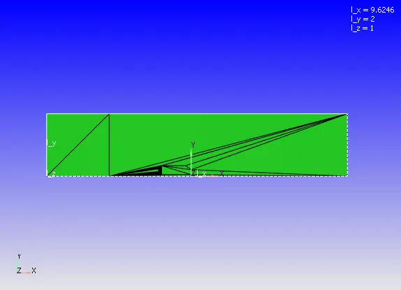
Diagnosis toolbar is used for geometry check-up.
In converge every part of the geometry is assumed to be triangle. The group of triangles are assigned to form a boundary. The boundaries are formed by using the following command. Geometry --> Boundary --> Flag --> Add boundary --> Create two boundaries --> Select the particular triangles and allot them to one region --> Apply.
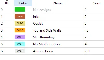
Then the normal are checked whether they are pointing inside the geometry where does the flow passes.
Case Setup:
- The application type is fixed with time based.
- Then click on Materials which is present in the right side of the window that is case setup tree and select the Predefined mixtures as Air.
i) Materials:
- Click on the Gas simulation and Global Transport parameter and retain the same values.
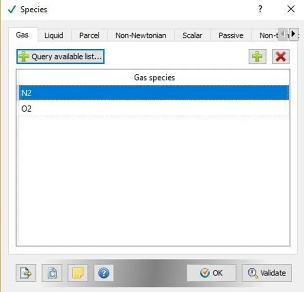
- Click on Species and then add O2 and N2.
ii) Simulation Parameters:
- Click on Run Parameters and under the solver tab choose the solver as Steady-State Solver. Set the simulation mode to Full Hydrodynamic and the gas flow solver as compressible.
- Since this is a transient simulation case setup, end time was calculated using the flow through time formula. Flow through time is the time taken by the fluid particles to travel from the inlet to outlet boundary with certain inlet velocity.
`v` = 40 m/s
Using the calculated inlet velocity, the flow through was calculated using the following formula.
Flow through time = Total Length of the wind Tunnel / Inlet Velocity
Therefore, Flow through time = `10/40`
Flow though time is approximately = 0.25 seconds.
As a best practice in transient flow simulation, the flow has to pass 4 times through the geometry.
Hence the end time was set with 4*0.25 = 1 second.
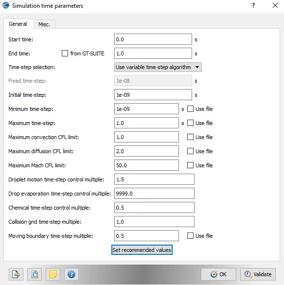
- Then under Solver Parameters retain the default settings.
iii) Initial Conditions and Events:
Regions and Initialisation:
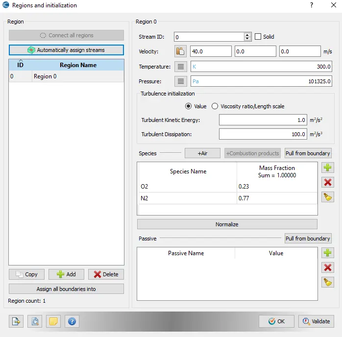
- Grouping the boundaries to form volumetric zones called region. This defines a volumetric region with initial conditions like initial pressure, initial temperature, velocity and species concentration.
- Under Regions and Initialisation, select add to create regions. Add a region and assign the velocity to be 40 m/s in X-direction. Add the species.
iv) Boundary Conditions:
Boundary:
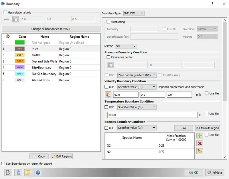
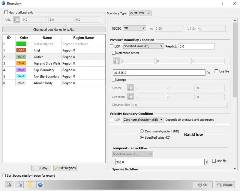
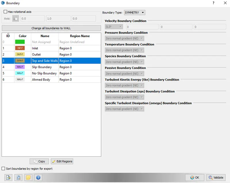
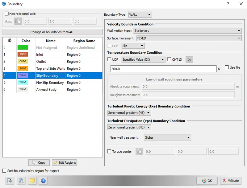
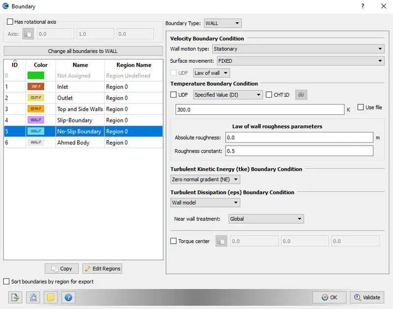
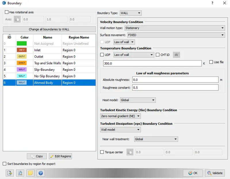
Under this parameter the boundaries have been defined and assigned with the following boundary conditions.
Inlet:
Outlet:
Top and Side Walls:
Slip Boundary:
No Slip Boundary:
Ahmed Body:
v) Physical Models:
Turbulence Modelling:
Then under the physical models check the turbulence modelling and set with Reynolds Averaged Navier-Stokes (RANS) and set the turbulence model with RNG K-epsilon.
vi) Grid Control:
Under grid control tab enable the Fixed Embedding option.
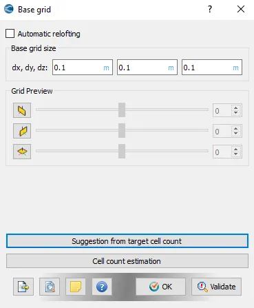
Then in the Grid Control parameter --> Base Grid --> Enter the size of the grid.
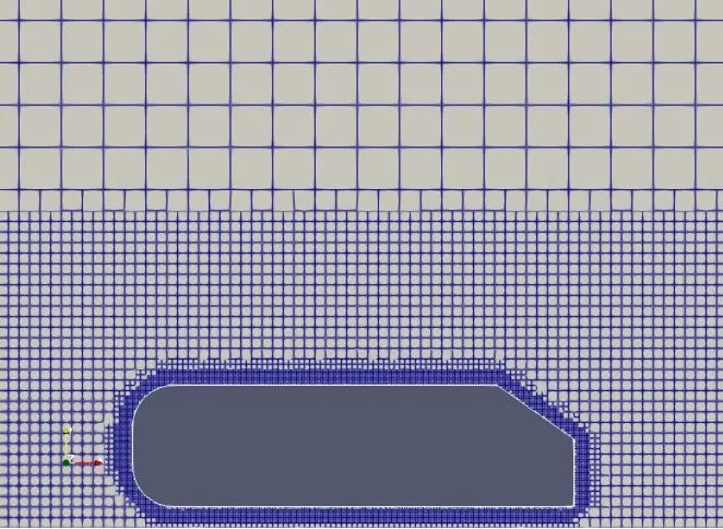
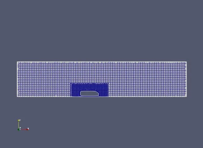
The size of the grid is assigned with 0.1 m. In order to have a correct approximation near the wall of the airfoil, fixed embedding parameter was used for the entire simulation time. The fixed embedding scale is important to observe the turbulence and flow separation near the airfoil wall. As we are using RNG K-epsilon model the y+ value should be greater than 30. In this project we have used the y+ value of 155 and calculated the first layer thickness and the scale value for fixed embedding.
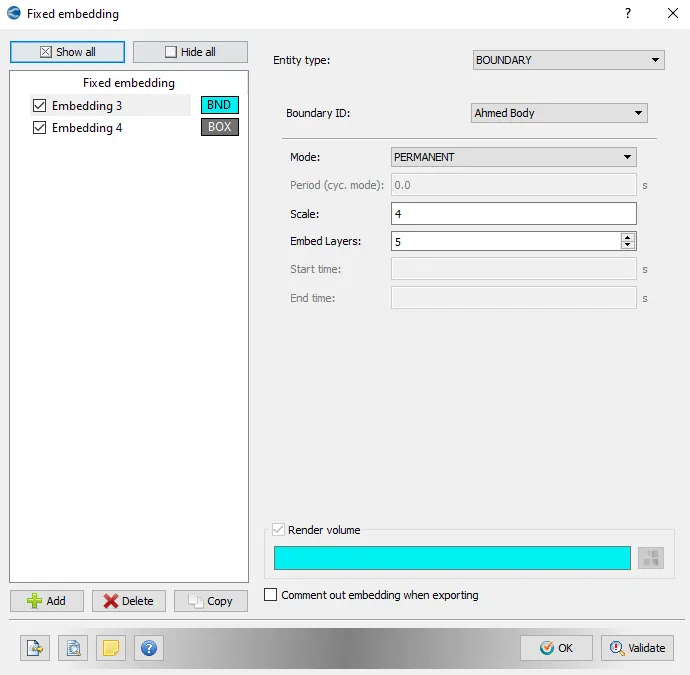
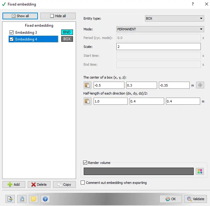
The fixed embedding can also be given for a specified region using Box Entity type. There will be wake region behind Ahmed body and in order to capture the results accurately in that region we again need finer mesh. Since there are no walls in that region, a BOX with above mentioned centre and half dimensions along 3 axes are created with scale 2 so that all the cells inside this box region are refined.
vii) Output/Post-Processing:
Then under Output/Post-Processing --> Post Variable Selection --> Under Combustion/Turbulence enable the y+ parameter and add the Mass fraction with O2 and N2
Then under the Output files --> Writing time intervals --> set the time interval for writing 3D output data files and time interval for writing restarting output.
Added to that under Output files --> Output Generation --> Wall Output --> Boundaries Only option is chosen which is important parameter for external aerodynamic simulation.
Then use CYGWIN to execute the CFD solver.
Then with the help of Converge CFD the post converting the output files to Paraview format is done.
Paraview is used for Post processing the results.
Post Processing:
Mesh:
Velocity Contour:
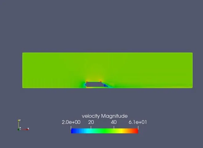
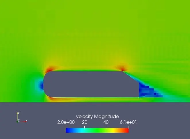
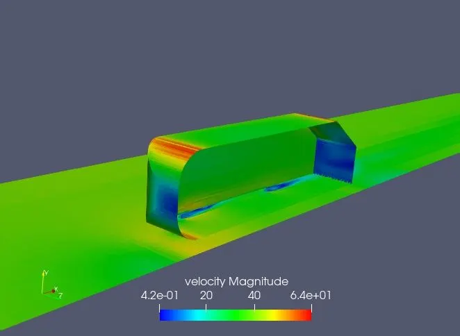
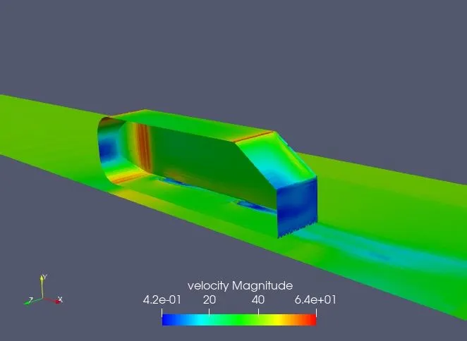
From the plot we could observe low pressure region formation at the front side of the Ahmed body. This is due to the stagnation of the fluid over the Ahmed body. When the stagnation occurs, the velocity is dropped and the pressure is increased. In the back end of the Ahmed body, we could observe the wake region as there is no way for the fluid to occupy the space when the body is in motion. The wake region formation is the main cause for the drag formation.
Pressure Contour:
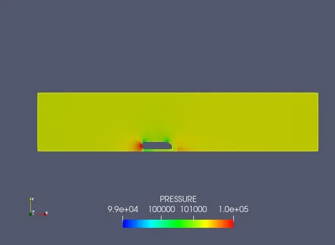
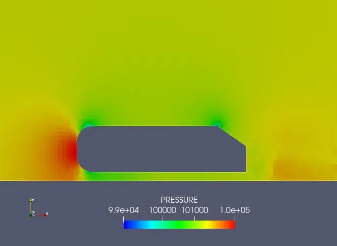
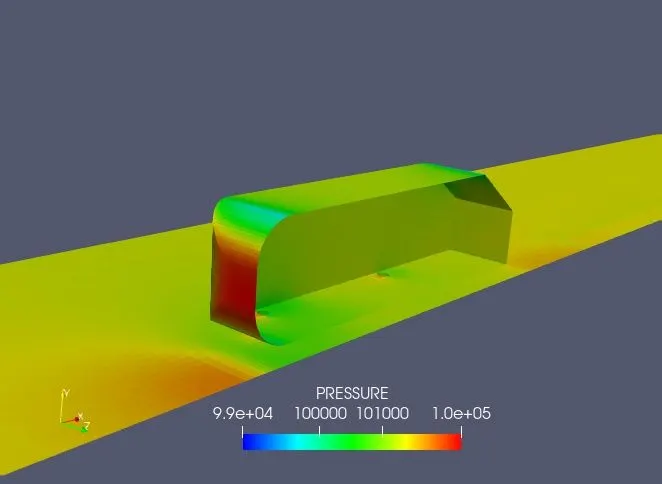
From the above contours, we could observe that the pressure increases drastically when the stagnation occurs which in turn decreases the velocity of the fluid. The high-pressure region is called as stagnation point.
Outlet Velocity:
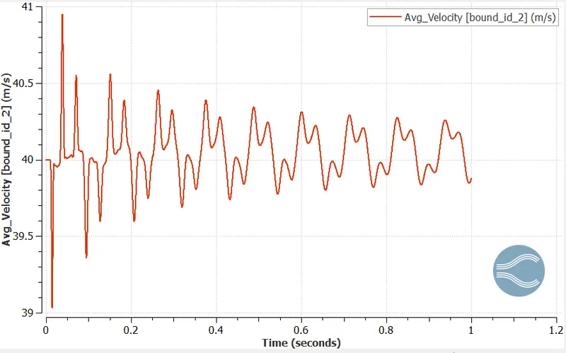
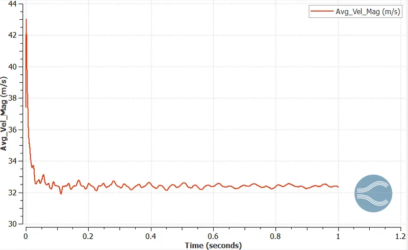
Average Velocity:
Pressure_Force_X (N):
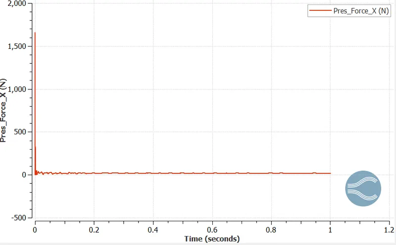
The above graph represents the pressure force in x-direction which is nothing but the drag produced by the Ahmed body at a free stream velocity of 40 m/s.
Pressure_Force_Y (N):
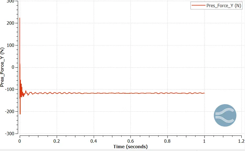
The above graph represents the pressure force in y-direction which is nothing but the lift produced by the Ahmed body at a free stream velocity of 40 m/s
Hence from the above plots we could attain the value of drag and lift forces which can be used for calculating the co-efficient of drag and lift.
`F_D=17.3725`
`F_L= -116.876`
`rho=1.1765(kg)/m^3`
`A=0.0446094`
`v=40`
Drag Calculation:
`C_D=(2*F_D)/(rho*v^2* A)`
`C_D = (2*17.3725)/(1.1765*40^2*0.0446094)`
`therefore C_D=0.413765255`
Lift Calculation:
`C_L=(2*F_L)/(rho*v^2* A)`
`C_L = (2*-116.876)/(1.1765*40^2*0.0446094)`
`therefore C_L = -2.783665451`
Paraview Surface Calculation:
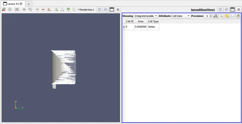
Paraview Drag and Lift Calculation:
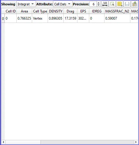
Drag force:
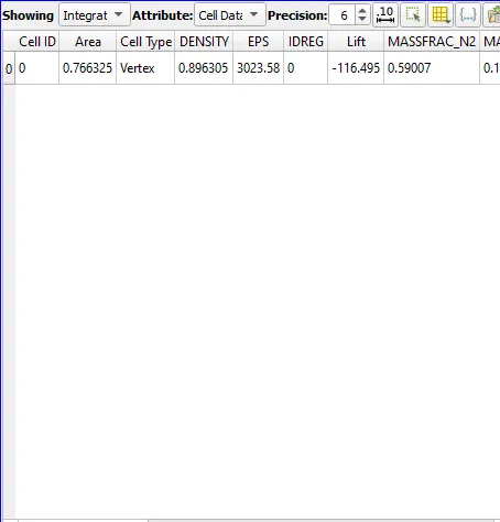
Lift Force:
Drag force = 17.3159
Lift Force = -116.495
`rho=1.1765(kg)/m^3`
`A=0.0446094`
`v=40`
Drag Calculation:
`C_D=(2*F_D)/(rho*v^2* A)`
`C_D = (2*17.3159)/(1.1765*40^2*0.0446094)`
`therefore C_D=0.412417199`
Lift Calculation:
`C_L=(2*F_L)/(rho*v^2* A)`
`C_L = (2*-116.495)/(1.1765*40^2*0.0446094)`
`therefore C_L = -2.774591077`
Experimental data and Simulation data comparison:
The results obtained from the simulation is cross-checked with experimental results. In the external flow over ahmed body experiment different line probes are placed at different x-location (flow-direction) and velocity along the y-direction (direction perpendicular to the flow direction) are plotted. Different x-location at which the line probes placed are -13 mm, -263 mm, 37 mm, 87 mm, -113 mm, -63 mm, 187 mm, 137 mm from the origin.
In paraview plot over line option is used and line probes are placed at above mentioned locations along x . direction and the velocity data obtained is plotted against the velocity data at same locations obatined from experimental results. Plots obtained are as shown below.
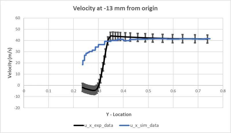
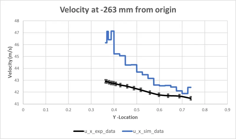
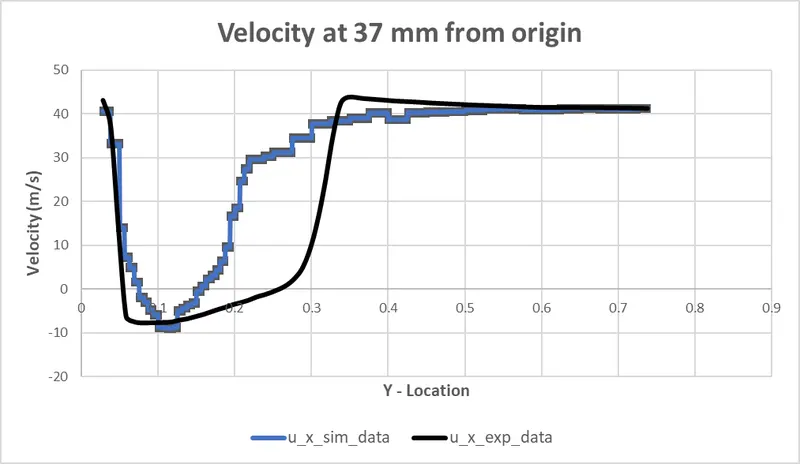
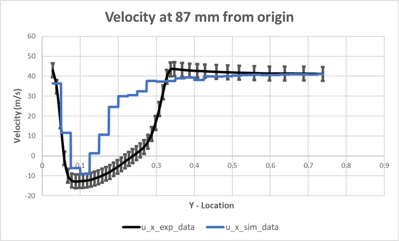
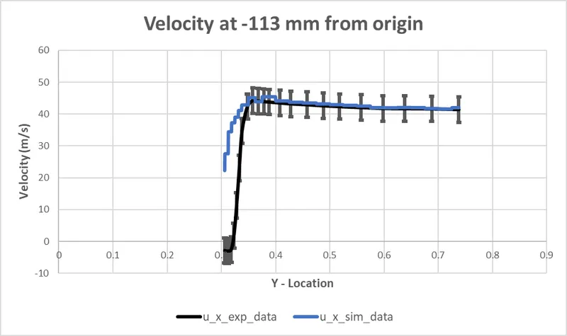
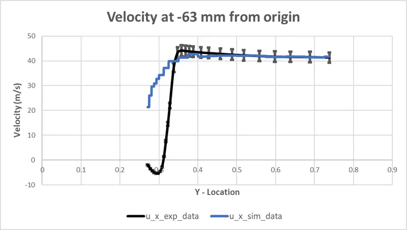
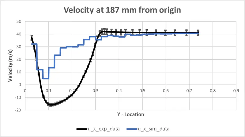
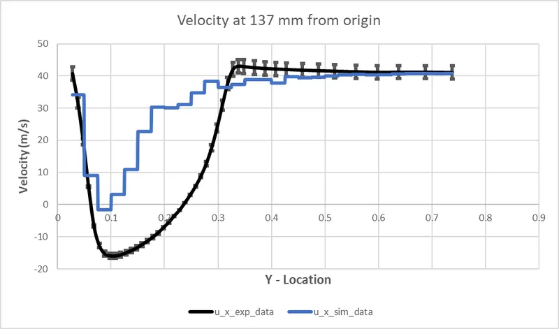
We can see some amount of error between the experimental and simulation date This is because our simulation is ran with coarser mesh and the cell sizes are big. The error would be reduced by making use of smaller cells but it would require lot more computational resource. But the current results obtained from our simulation are satisfatory.
Plots which are having positive x axis are just behind the Ahmed body which is wake region charcaterised by low pressure and drop in velocity.
Animation Videos:
Velocity Animation - https://youtu.be/3cBEd-QAmD4
Pressure Animation - https://youtu.be/HX3Yy8Cf8BM
Conclusion:
- The flow around the Ahmed body was simulated using CONVERGE CFD in which the Ahmed body was modelled using CATIA V5R20 CAD software.
- The virtual wind tunnel was setup by calculating the boundary layer thickness parameters.
- The 35 degree slant angle of Ahmed body is compared with experimental data and simulation data.
- The contours for velocity and pressure profiles are displayed.
- From the contour plot we could conclude that the pressure is more on the front side of the Ahmed body, that happened because of stagnation point. A wake region could be observed at the backside of the Ahmed body in which there is no way for the fluid to reach the region.
- The velocity is low on the backside of the Ahmed body and the flow is recirculated behind the body because of the slant angle.
- There is more difference in the experimental data and the simulation data because of the low number cell count used in simulation. In order to get more accurate results, more computational time and power are required.
- The drag and lift force is calculated on both converge studio and paraview platform and the co-efficient of drag and lift is calculated using formulas.
- The negative lift force represents that in the ahmed body the lift force is acting downwards.
- The way to calculate the aerodynamic forces using paraview are studied.
- The procedure for the comparison of the experimental data with the simulation data are discussed.