Week 5.1 - Mid term project - Solving the steady and unsteady 2D heat conduction problem

Week 5.1 - Mid term project - Solving the steady and unsteady 2D heat conduction problem:

Aim:

• To solve the 2D Steady state heat conduction equation by using point iterative technique (Jacobi,Gauss-seidel,Successive over-relaxation)
• To solve the 2D transient/unsteady heat conduction equation by using explicit and implicit method.

The 2D heat conduction equation is of two types:

i) Steady state

ii)unsteady state

Governing equation:

2D steady state heat conduction equation is represented as,

`(del^2T)/(delx^2)+(del^2T)/(dely^2)=0`

Since it is a steady state equation the time term is zero and diffusivity is constant.

2D Unsteady state heat conduction equation is represented as,

`(delT)/(delt)+alpha*(del^2T)/(delx^2)+(del^2T)/(dely^2)=0`

Here the equation is hyperbolic as the time/information is traveeling in only one direction.

i) 2D steady state heat conduction equation:

`(del^2T)/(delx^2)+(del^2T)/(dely^2)=0`

Where 'T' is temperature, x and y are special co-ordinates.

`T_p=1/k*((T_l+T_r)/(delx^2))+((T_T+T_B)/(dely^2))`

If the above equation is represented in nodes(i,j), it is represnted as,

`T_(i,j)=1/k*((T_(i-1,j)+T_(i+1,j))/(delx^2))+((T_(i,j-1)+T_(i,j+1))/(dely^2))`

MATLAB code for Steady State heat conduction equation:

Main code:

%Steady State condition
clear all
close all
clc

%inputs
%Number of grid points along x and y directions
nx=10;
ny=10;
x=linspace(0,1,nx);
dx=x(2)-x(1);
y=linspace(0,1,ny);
dy=y(2)-y(1);
t=300*ones(nx,ny);

%applying boundary conditions
t(1,:)=600;
t(end,:)=900;
t(:,1)=400;
t(:,end)=800;

method=0;
[xx,yy]=meshgrid(x,y);
K=(2*((dx^2+dy^2)/(dx^2*dy^2)));
error=9e9;
tol=1e-4;
told=t;
%told1=t;
%told2=t;
%told3=t;
t_initial=t;
iter=1;
%j_iter=1;
%gs_iter=1;
%sor_iter=1;
w=1.1;
method=input('Enter the method number 1.Jacobi 2.Gauss Seidel 3.SOR');
while error>tol
    for i=2:nx-1
    for j=2:nx-1
      if (method==1)
      t(i,j)=jacobi(told,i,j);
      elseif (method==2)
      t(i,j)=GS(t,told,i,j);
      elseif (method==3)
      t(i,j)=SOR(t,told,i,j);
      end
    end
    end
a=((t-told));
b=max(max(a));

error=b;
told=t;
iter=iter+1;

contourf(x,y,t,'showtext','on')
colormap(jet)
colorbar
set(gca,'YDIR','reverse')

xlabel('X axis')
ylabel('Y axis')
title(sprintf('2D steady state analysis (Jacobi) for %d Number of iterations',iter))
pause(0.003)
end
        

Function code:

%Function for Jacobi method:
function out=jacobi(told,i,j);
out=0.25*((told(i,j-1)+told(i,j+1)+told(i-1,j)+told(i+1,j)));
end

%Function for Gauss Seidel method:
function out=GS(t,told,i,j);
out=0.25*((t(i,j-1)+told(i,j+1)+t(i-1,j)+told(i+1,j)));
end

%Function for SOR method:
function out=SOR(t,told,i,j);
w=1.1;
out=(1-w)*told(i,j)+ w*(0.25*(t(i,j-1)+told(i,j+1)+t(i-1,j)+told(i+1,j)));
end

Plots:

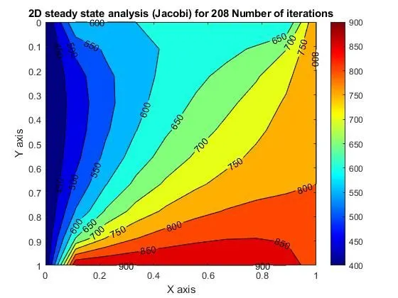
For Jacobi method:

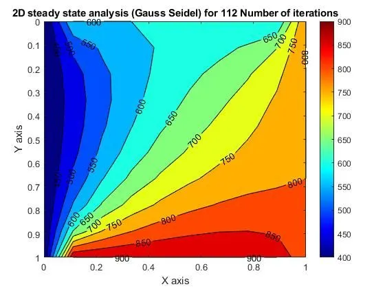
For Gauss Seidel method:

For SOR method:

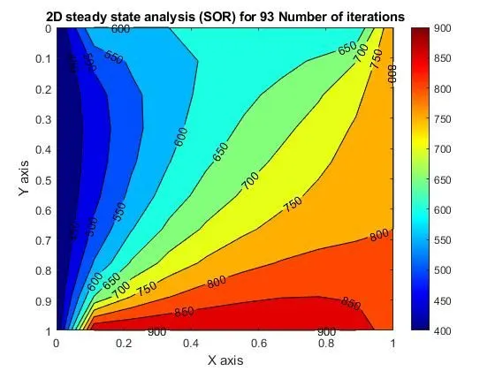
From the above plots we could predict that SOR method is the fastest method as it solves for lesser no of iterations when compared with the other methods.

2D Unsteady state heat conduction equation:

2D Unsteady state heat conduction equation is represented as,

`(delT)/(delt)+alpha*(del^2T)/(delx^2)+(del^2T)/(dely^2)=0`

Here the equation is hyperbolic as the time/information is traveeling in only one direction.

As already mentioned the unsteady equation can be solved using two different methods:

i)Explicit

ii)Implicit

MATLAB code for Unsteady State heat conduction equation:

Explicit method:

%UnSteady State condition by Explicit method:
clear all
close all
clc

%inputs
%Number of grid points along x and y directions
nx=10;
ny=10;
x=linspace(0,1,nx);
dx=x(2)-x(1);
y=linspace(0,1,ny);
dy=y(2)-y(1);
t=300*ones(nx,ny);

%applying boundary conditions
t(1,:)=600;
t(end,:)=900;
t(:,1)=400;
t(:,end)=800;

method=0;
[xx,yy]=meshgrid(x,y);
k=(2*((dx^2+dy^2)/(dx^2*dy^2)));
error=9e9;
tol=1e-4;
told=t;
told1=t;
told2=t;
told3=t;
t_initial=t;
iter=1;
j_iter=1;
gs_iter=1;
sor_iter=1;
w=0;
a1=1.5;
t_tot=10;
dt=2;
nt=t_tot/dt;
k=a1*dt/(dx^2);
%CFL number to check for stability condition
cfl=a1*dt/(dx^2);

method=input('Enter the method 1.Explicit');

if (method==1)
    a1=0.02;
    t_tot=10;
    dt=0.1;
    nt=t_tot/dt;
    %nt=30;
    k=a1*dt/(dx^2);
    cfl=a1*dt/(dx^2);
    %Explicit scheme
    for o=1:nt
        for i=2:nx-1
            for j=2:ny-1
                term1=(told(i-1,j)-(2*told(i,j))+told(i+1,j));
                term2=(told(i,j-1)-(2*told(i,j))+told(i,j+1));
                t(i,j)=told(i,j)+k*(term1+term2);
            end
        end
        error=max(max(abs(told-t)));
        told=t;
    end

%Plot
contourf(x,y,t,'showtext','on')
colormap(jet)
colorbar
set(gca,'YDIR','reverse')

xlabel('X axis')
ylabel('Y axis')
title(sprintf('2D Unsteady Heat conduction equation by Explicit method'));
pause(0.003)
end

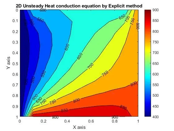
Plot:

CFL Value: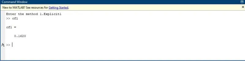

Implicit method:

%UnSteady State condition by Explicit method:
clear all
close all
clc

%inputs
%Number of grid points along x and y directions
nx=10;
ny=10;
x=linspace(0,1,nx);
dx=x(2)-x(1);
y=linspace(0,1,ny);
dy=y(2)-y(1);
w=1.2;
t=ones(nx,ny)*298;

%applying boundary conditions
t(1,:)=600;
t(end,:)=900;
t(:,1)=400;
t(:,end)=800;

alpha=1.4;
dt=0.001;

%defining k1 nad k2
k1=alpha*(dt/dx^2);
k2=alpha*(dt/dy^2);

told=t;
t_initial=t;

%[xx,yy]=meshgrid(x,y);
%k=(2*((dx^2+dy^2)/(dx^2*dy^2)));
error=9e9;
tol=1e-4;

for iterative_solver=1:3
    nt=1:1400;
    error=9e9;
    tol=1;
    tic;

%iterative_solver=1:3;
iter=1;
while error>tol
    for i=2:nx-1
        for j=2:ny-1
            term1=1/(1+2*k1+2*k2);
            term2=k1*term1;
            term3=k2*term1;
            if iterative_solver==1
                t(i,j)=((told(i,j)*term1)+(term2*(t(i-1,j)+t(i+1,j))+(term3*(t(i,j-1)+t(i,j+1)))));
            elseif iterative_solver==2
                   t(i,j)=((told(i,j)*term1)+(term2*(t(i-1,j)+told(i+1,j))+(term3*(t(i,j-1)+told(i,j+1)))));
            elseif iterative_solver==3
                   t(i,j)=(1-w)*told(i,j)+w*(((told(i,j)*term1)+(term2*(t(i-1,j)+told(i+1,j))+(term3*(t(i,j-1)+told(i,j+1))))));
            end
        end
        error_n=max(abs(told-t));
        error=max(error_n);
        told=t;
        iter=iter+1;
    end
end
time=toc;

%plot

if iterative_solver==1
    figure(1)
    contourf(x,fliplr(y),t);
    [C,h]=contourf(x,fliplr(y),t);
    colorbar;
    colormap(jet);
    clabel(C,h);
    text=sprintf('JACOBI Method for n iteration number = %d; t compuational time: %0.4f',iter,time);
    title(text);
    told=t_initial;
    t=t_initial;

elseif iterative_solver==2
    figure(2)
    [C,h]=contourf(x,fliplr(y),t);
    colorbar;
    colormap(jet);
    clabel(C,h);
    text=sprintf('GS Method for n iteration number = %d; t compuational time: %0.4f',iter,time);
    title(text);
    told=t_initial;
    t=t_initial;

else 
    figure(3)
    [C,h]=contourf(x,fliplr(y),t);
    colorbar;
    colormap(jet);
    clabel(C,h);
    text=sprintf('SOR Method for n iteration number = %d; t compuational time: %0.4f',iter,time);
    title(text);
    told=t_initial;
    t=t_initial;
end
end


            

         

Plots:

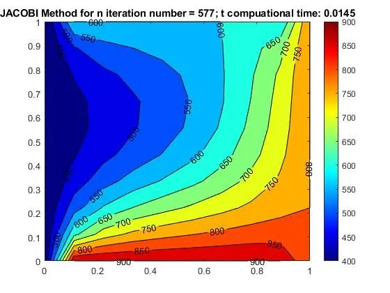
Jacobi method:

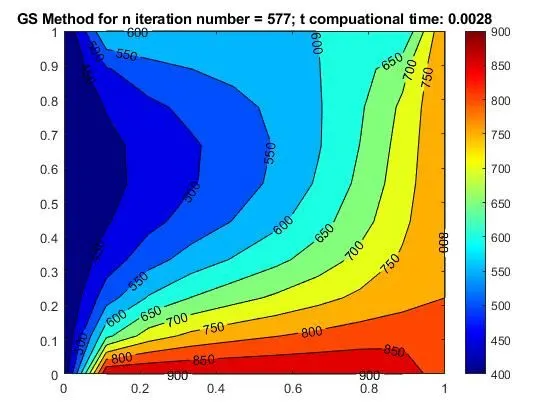
Gauss Seidel method:

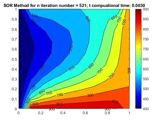
SOR method:

Result:

While comparing both the Explicit and implicit method's results, it is predicyed that Explicit method is much quicker than the implicit method. The explicit method takes 201 iterations whereas the implicit method takes 577,577,521 iterations for Jacobi, Gauss Seidel, SOR methods respectively. Coming to the implicit method SOR is the fastest method while comparing it with Jacobi and Gauss Seidel. But the implicit method is more accurate as it uses various iterative solvers.