Week 3.2 - Simulating a 2nd order ODE system of a simple pendulum

The way the pendulum moves depends on the Newtons second law. When this law is written down, we get a second order Ordinary Differential Equation that describes the position of the "ball" w.r.t time.

Similarly, there are hundreds of ODEs that describe key phenomena and if you have the ability to solve these equations then you will be able to simulate any of theses systems.

Objective:

To write a program that solves the following ODE. This ODE represents the equation of motion of a simple pendulum with damping.

This equation represents the equation of motion of a simple pendulum with damping:

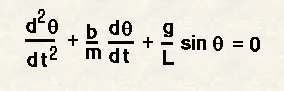
In this equation

g = gravity in m/s2,

L = length of the pendulum in m,

m = mass of the ball in kg,

b=damping coefficient.

With the given initial conditions,

L=1 metre,

m=1 kg,

b=0.05.

g=9.81 m/s2

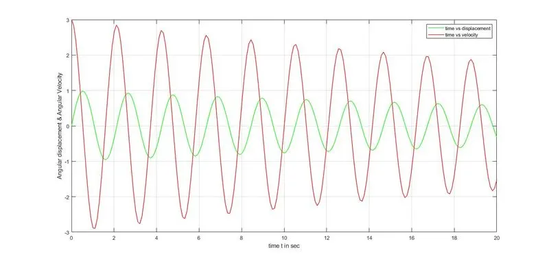
we have to simulate the motion between the time range 0-20 seconds for angular displacement =0 and anglular velocity =3 rad/sec^2 at time t=0.

MATLAB Code:

Function code:

function xdot=pendulum_2nd_order(t,x)
%damping co-efficient
b=0.05;
%mass
m=1;
%gravity
g=9.81;
%length
L=1;
xdot=zeros(2,1);
xdot(1)=x(2);%Angular dispalcement
xdot(2)=(-b/m)*x(2)-(g/L)*sin((x(1)));%Angular Velocity
end 

Main Code:

clear all
close all
clc
%inputs
L=1;
t=linspace(0,20,200);
x0=[0 3];
%Solving ODE
[t,x]=ode45('pendulum_2nd_order',t,x0);

%Plotting and tracing of angular velocity and angular displacement

plot(t,x(:,1),'color','g','linewidth',1);
xlabel('time t in sec');
ylabel('Angular displacement & Angular Velocity');
hold on;
plot(t,x(:,2),'color','r','linewidth',1);
legend('time vs displacement','time vs velocity')
grid on;

%Animation

X0=0;
Y0=0;
ct=1;%counter represents each and every frame
for i=1:length(t)
    X1=L*sin(x(i,1));
    Y1=-L*cos(x(i,1));
   
figure(2)
plot([-1 1],[0 0],'linewidth',6,'color','g');
axis([-2 2 -2 2]);
line([X0 X1], [Y0 Y1],'linewidth',2,'color','b');
hold on;
plot(X0,Y0,'o','markersize',3,'markerfacecolor','y');
plot(X1,Y1,'o','markersize',20,'markerfacecolor','r');
title('Damping of simple pendulum');
legend('Support rod','length of pendulum','fixed point','Bod of pendulum');
grid on;
hold off;
M(ct)=getframe(gcf);
    ct=ct+1;
end

movie(M)
videofile=VideoWriter('simplependulum.avi','uncompressed AVI');
open(videofile)
writerVideo(videofile,M)
close(videofile)

Results:

YOUTUBE Link of the video that represents Simple Pendulum Motion:

https://youtu.be/73lkn4k-8gU

Relation between Angular Displacement and Angular Velocity: