Week 5.3 - Mid term project - Stability analysis in the unsteady problem

Week 5.3 - Mid term project - Stability analysis in the unsteady problem:

Aim:

To perform stability analysis in the unsteady problem.

The 2D heat conduction equation is of two types:

i) Steady state

ii)unsteady state

Governing equation:

2D steady state heat conduction equation is represented as,

`(del^2T)/(delx^2)+(del^2T)/(dely^2)=0`

Since it is a steady state equation the time term is zero and diffusivity is constant.

2D Unsteady state heat conduction equation is represented as,

`(delT)/(delt)+alpha*(del^2T)/(delx^2)+(del^2T)/(dely^2)=0`

Here the equation is hyperbolic as the time/information is travelling in only one direction.

i) 2D steady state heat conduction equation:

`(del^2T)/(delx^2)+(del^2T)/(dely^2)=0`

Where 'T' is temperature, x and y are special co-ordinates.

`T_p=1/k*((T_l+T_r)/(delx^2))+((T_T+T_B)/(dely^2))`

If the above equation is represented in nodes(i,j), it is represnted as,

`T_(i,j)=1/k*((T_(i-1,j)+T_(i+1,j))/(delx^2))+((T_(i,j-1)+T_(i,j+1))/(dely^2))`

ii)2D Unsteady state heat conduction equation:

2D Unsteady state heat conduction equation is represented as,

`(delT)/(delt)+alpha*(del^2T)/(delx^2)+(del^2T)/(dely^2)=0`

Here the equation is hyperbolic as the time/information is traveeling in only one direction.

As already mentioned the unsteady equation can be solved using two different methods:

i)Explicit

ii)Implicit

Assumptions made to solve the transient-state equation are as follows:

1) The domain itself is a square unit.

2) We are considering that the points along the x-direction are equal to the numbers of points in the y-direction by assuming nx=ny

3) Boundary Conditions are assurned as follows:

• Left sided Boundary-400K
• Right-sided Boundary-800K
• Top-sided Boundary-600k
• Bottom-sided Boundary-900K

4)Tolerance is given as le-4

A solution can simplest turn out to be unstable if there are errors in it. As we discretize our equation, we're approximating the terms and at the same time as approximating we have a tendency to disregard the terms which might be causing truncation errors.

1. Consistency and Stability are of the maximum critical elements essential to recollect at the same time as deriving a numerical scheme.

2. As the errors which might be generated in the numerical approximations are integrated into the answer, those errors get magnified with respect to time and sooner or later make the solutions attain unstable situations which can not be relied on in addition for real-international applications.

3. Hence, errors have to be bounded and shouldn't grow much further.

Role of CFL number:

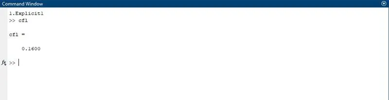
It is necessary condition for convergence while solving certain PDE numerically. It arises in the numerical analysis of explicit schemes. The time step must be less than a certian time in explicit time marching computer simulation, otherwise simulation produces in accurate results.

CFL value is calculated using the given formula

cfl=(c*dt)/dx;

MATLAB Code:

Unsteady Explicit scheme:

%UnSteady State condition by Explicit method:
clear all
close all
clc

%inputs
%Number of grid points along x and y directions
nx=10;
ny=10;
x=linspace(0,1,nx);
dx=2.5e-2;
y=linspace(0,1,ny);
dy=2.5e-2;
t=450*ones(nx,ny);

%applying boundary conditions
t(1,:)=600;
t(end,:)=900;
t(:,1)=400;
t(:,end)=800;

%method=0;
[xx,yy]=meshgrid(x,y);
%k=(2*((dx^2+dy^2)/(dx^2*dy^2)));
error=9e9;
tol=1e-4;
told=t;

a1=0.005;
dt=1e-2;
iter=0;
k1=a1*dt/(dx^2);
k2=a1*dt/(dy^2);
%CFL number to check for stability condition
cfl=k1+k2;

method=input('1.Explicit');

if (method==1)
    tic
    %Explicit scheme
    while(error>tol)
        for i=2:nx-1
            for j=2:ny-1
                t(i,j)=(1-2*k1-2*k2)*told(i,j)+k1*(told(i-1,j)+told(i+1,j))+k2*(told(i,j-1)+told(i,j+1));
            end
        end
        error=max(max(abs(t-told)));
        told=t;
        iter=iter+1;
    end
time=toc;
%Plot
contourf(x,y,t,'showtext','on')
colormap(jet)
colorbar
set(gca,'YDIR','reverse')

xlabel('X axis')
ylabel('Y axis')
title(sprintf('2D Unsteady Heat conduction equation by Explicit method with %d number of iterations and t compuational time: %0.4f',iter,time));
pause(0.005)
end

Plot:

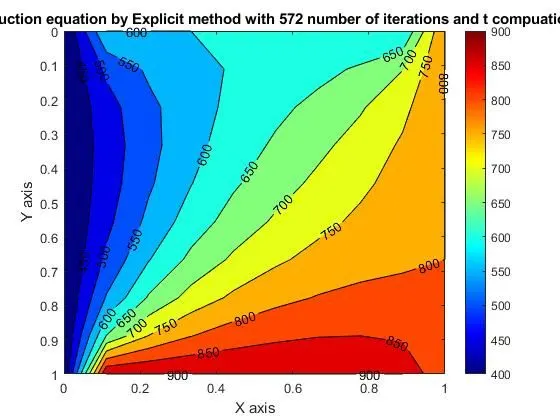
Explanation:

i.In the case of explicit scheme, it is not unconditonally stable when compared to the other schemes and hence we have to make sure that the size of the timesteps is relatively smaller for this scheme to maintain stability.

ii.The overall computing time increases due to decrease in the size of the timestep.

iii.From the above results we can observe that it took 572 iterations for the solution to reach convergence

iv.Hence we have to make sure that the CFL value is lower than or equal to 0.50 for the solution to remain stable.

v.The CFl value that we are getting for this problem is 0.1600 whichis sufficiently lower than 0.50.

vi. The solution reaches convergence a long as CFL is less than equal to 0.48 but after that the solution enters into divergence an blows up.

Unsteady Implicit scheme:

%UnSteady State condition by Implicit method:
clear all
close all
clc

%inputs
%Number of grid points along x and y directions
nx=10;
ny=10;
t=450*ones(nx,ny);

x=linspace(0,1,nx);
y=linspace(0,1,ny);

%applying boundary conditions
t(1,:)=600;
t(end,:)=900;
t(:,1)=400;
t(:,end)=800;

%storing a copy
told=t;
t_initial=t;
t_prev=t;

%grid spacing
dx=1e-2;
dy=1e-2;

%timestep
dt=1e-2;

%Thermal diffusivity
alpha=0.015;

%defining k1 and k2
k1=alpha*(dt/dx^2);
k2=alpha*(dt/dy^2);

%iterative solvers=1) Jacobi 2)Gauss Seidel 3)SOR

%1. Jacobi solver
error=9e9;
tol=1e-4;
conv=9e9;
jac_iter=0;
jac_time_iter=0;

%time loop
while conv>tol
    %Space loop
    while error>tol
    for i=2:nx-1
        for j=2:ny-1
                t(i,j)=(1+2*k1+2*k2)^-1*(t_prev(i,j)+k1*(told(i-1,j)+told(i+1,j))+k2*(told(i,j-1)+told(i,j+1)));
        end
    end
        error_n=max(abs(t-told));
        error=max(error_n);
        told=t;
        jac_iter=jac_iter+1;
    
figure(1)
contourf(flipud(t),'ShowText','ON')
title(sprintf('transient implicit Jacobi solver iterations= %d ntime iterations =%d',jac_iter,jac_time_iter));
pause(0.005)
    end
conv=max(max(abs(t-t_prev)));
t_prev=t;
jac_time_iter=jac_time_iter+1;
error=9e9;
end
colorbar
%reinitialising
t=t_initial;
told=t;
t_prev=t;
error=9e9;
conv=9e9;


%2. Gauss Seidel solver
gs_iter=0;
gs_time_iter=0;

%time loop
while conv>tol
    %Space loop
    while error>tol
    for i=2:nx-1
        for j=2:ny-1
                t(i,j)=(1+2*k1+2*k2)^-1*(t_prev(i,j)+k1*(t(i-1,j)+told(i+1,j))+k2*(t(i,j-1)+told(i,j+1)));
        end
    end
        error_n=max(abs(t-told));
        error=max(error_n);
        told=t;
        gs_iter=gs_iter+1;
    
figure(2)
contourf(flipud(t),'ShowText','ON')
title(sprintf('transient implicit GS solver iterations= %d ntime iterations =%d',gs_iter,gs_time_iter));
pause(0.005)
    end
conv=max(max(abs(t-t_prev)));
t_prev=t;
gs_time_iter=gs_time_iter+1;
error=9e9;
end
colorbar
%reinitialising
t=t_initial;
told=t;
t_prev=t;
error=9e9;
conv=9e9;


%SOR solver
sor_iter=0;
sor_time_iter=0;
omega=1.5;

%time loop
while conv>tol
    %Space loop
    while error>tol
    for i=2:nx-1
        for j=2:ny-1
                tgs(i,j)=(1+2*k1+2*k2)^-1*(t_prev(i,j)+k1*(t(i-1,j)+told(i+1,j))+k2*(t(i,j-1)+told(i,j+1)));
                t(i,j)=(1-omega)*told(i,j)+omega*(tgs(i,j));
        end
    end
        error_n=max(abs(t-told));
        error=max(error_n);
        told=t;
        sor_iter=sor_iter+1;
    
figure(3)
contourf(flipud(t),'ShowText','ON')
title(sprintf('transient implicit SOR solver iterations= %d ntime iterations =%d',sor_iter,sor_time_iter));
pause(0.005)
    end
conv=max(max(abs(t-t_prev)));
t_prev=t;
sor_time_iter=sor_time_iter+1;
error=9e9;
end
colorbar
%reinitialising
t=t_initial;
told=t;
t_prev=t;
error=9e9;
conv=9e9;

Plots:

Implicit:

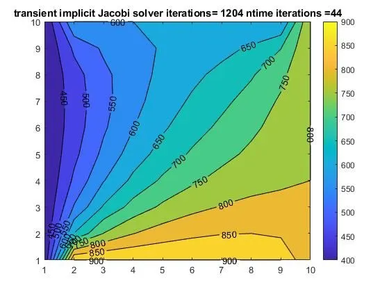
Jacobi method:

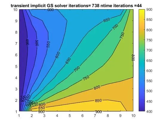
Gauss Seidel method:

SOR method:

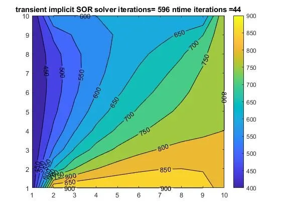
Explanation:

1. In the case of the Implicit Scheme, higher values of 'dt' give unconditionally stable solutions irrespective of the resultant reduction in the degree of accuracy provided by it.

2. With the increase in the value of 'dt' the solutions are experiencing an increase in the truncation error value which results in bringing more errors and reduces the accuracy of the overall solution.

3. Here, the value of 'dt' is assumed as 1e-2 and the output remains stable for that value which would have been impossible in the case of an explicit scheme