Modeling and Simulation of flow around an Ahmed Body
I. Aim: Aerodynamic flow simulation around an Ahmed body using Converge CFD.
II. Introduction:
The Ahmed body is a generic car body (a simplified vehicle model). The flow of air around the Ahmed body captures the essential flow features around an automobile and was first defined and characterized by Ahmed [1] in his experimental work. Ahmed body is of a simple shape, which allows us to capture characteristic features that are relevant to bodies in the automobile industry.
The Ahmed body is a benchmark model widely used in the automotive industry for validating simulation tools because complexly shaped cars are very challenging to model and it’s difficult to quantify the aerodynamic drag computationally.
The simple geometrical shape of the Ahmed body has a length of 1.044 meters, a height of 0.288 meters, and a width of 0.389 meters. It also has 0.05-meter cylindrical legs attached to the bottom of the body and the rear surface has a slant that falls off at angles in the range of 25-40 degrees. The dimensions of the geometry used in the current analysis is shown below:
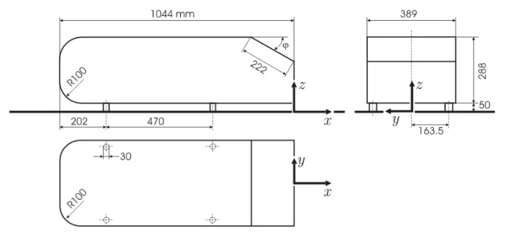
Figure 1: Dimensions of the Ahmed Body (`phi`= 35 degrees).
Drag coefficient in cars:
The resistance experienced by a fluid environment to an object in motion is quantified in terms of drag force. Generally, the forces acting on an object in motion or a stationary object in a flowing fluid are classified into drag and lift forces. The component parallel to the fluid flow direction is called the drag force and the forces perpendicular to the fluid flow direction are called lift forces.
The drag force acting on a body is given by the formula:
`F_d=1/2C_dρAV^2`
where, F_d = Drag force in Newtons
C_d= drag coefficient
ρ = Density of the fluid in kg/m^3
A = frontal area of the object in m^2
V = fluid velocity/object velocity in m/s.
The lift force acting on a body is given by the formula:
`F_l=1/2C_lρAV^2`
where, F_l= lift force in Newtons
C_l = lift coefficient
ρ = Density of the fluid in kg/m^3
A = frontal area of the object in m^2
V = fluid velocity/object velocity in m/s.
Generally, ground vehicles(ex: cars) experience lift forces rarely while in motion, hence the study of drag forces on automobiles is important. The drag coefficient is a nondimensional way of expressing drag force, and it varies for different objects and also depends on the flow Reynolds number.
The lower the drag coefficient of an object, the less aerodynamic or hydrodynamic drag occurs. In terms of a car, the lower the drag coefficient, the more efficient the car is. As well as affecting the top speed of a vehicle, the drag coefficient also affects the handling. Cars with a low drag coefficient are sought after, but decreasing the drag drastically can reduce the downforce and lead to a loss in road traction and a higher chance of car accidents. The drag coefficient value ranges from 0.3-0.35 in most commercial cars. The value may be higher in SUVs and will be lesser than 0.3 in streamlined cars[2].
In this project, the 3D numerical analysis of flow around the Ahmed body is carried in Converge CFD and the results are compared with experimental data from [3].
III. Objectives:
1. Perform a steady-state simulation of flow over an Ahmed body and compare the results with experimental data.
2. Refine the grid to obtain accurate results
V: Solving & Modelling approach:
3D steady-state CFD analysis of flow around an Ahmed body with slant angle (ϕ = 35 degrees) case is set up in ConvergeCFD and then running the solution in CYGWIN terminal. Atmospheric air is used as the working fluid. Postprocessing is done using ConvergeCFD and ParaView.
1. Geometry/Domain:
The Ahmed body geometry is first created in SpaceClaim direct modeler with appropriate dimensions. The dimensions used for the geometry as well as the generated geometry are shown in the below images:
| Geometry Dimensions | Ahmed Body Geometry |
|
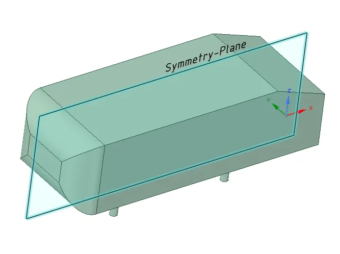 |
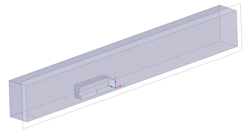
Since the Ahmed body is symmetrical about the mid-section along the XZ-plane, the geometry is split into two sections about the symmetry plane as shown in the above image. This will greatly reduce the computational time. Only half of the geometry is considered for the analysis and a flow domain is created around the Ahmed body using the enclosure option in SpaceClaim as shown below:
| Flow-Domain | Imported domain in Converge-CFD |
 |
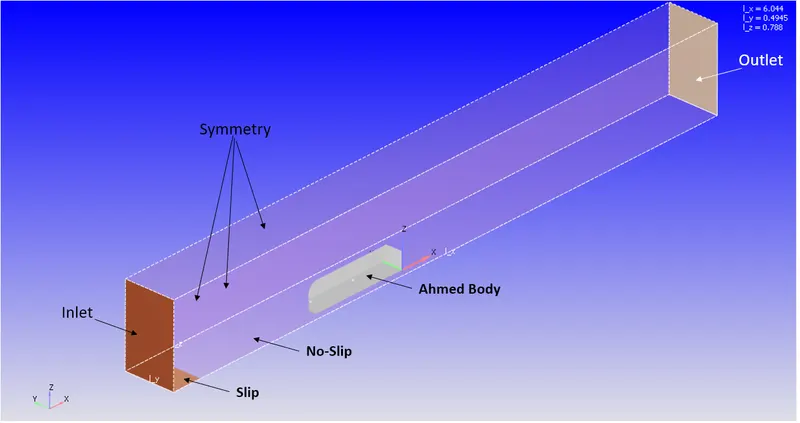 |
The created domain is then saved as .stl format file , which is imported in Converge CFD for setting up the analysis.
2. Boundary Flagging:
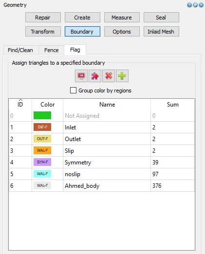
The boundary zones in ConvergeCFD are created by flagging boundaries. This can be done by creating boundary flags in the boundary tab as shown below:
3. Case setup:
After assigning boundary zones as mentioned above, the solution case setup is to be done. ConvergeCFD has a dedicated menu to completely set up the solution. Details are as follows:
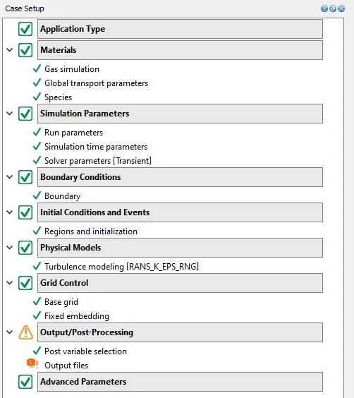
In the application type option, Time-based is selected.
- The materials option are selected as shown in the below images:
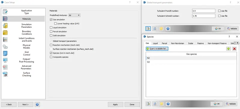
Air at atmospheric conditions is chosen as the working fluid. The following are properties of air used:
Density = 1.2 kg/m^3
Dynamic Viscosity = 1.86E-07 Pa-s.
- Simulation Parameters:
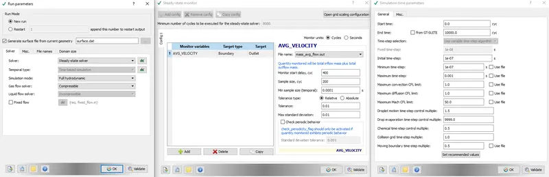
The flow over the airfoil is simulated using a steady-state solver by selecting steady-state solver option and the respective setting for the solver are shown below:
- Boundary Conditions:
The boundary zones are applied with boundary conditions in this step. The inlet flow velocity is taken as 40 m/s and the air properties at the atmospheric condition of 1 Bar pressure and 300 K temperature.
The applied boundary conditions are as follows:
| Boundary Zone | Boundary condition |
| Inlet |
Inflow (Dirichlet BC's) -Velocity = 40 m/s along x-direction -Temperature = 300 K - Species - O2 = 0.77, N2 - 0.23 |
| Outlet |
Outflow (Dirichlet BC's) - Pressure = 101325 Pa Neuman BCs - zero normal gradient Velocity -Backflow temperature =300 K |
| Symmetry |
Symmetry |
| noslip | no-slip |
| slip | slip |
| Ahmed_body |
Wall -Stationary, fixed, Law of Wall, Neuman conditions |
The above boundary conditions can be defined only after defining a region in the Initial conditions and Events section of the case setup with velocity in the region the same as inlet velocity.
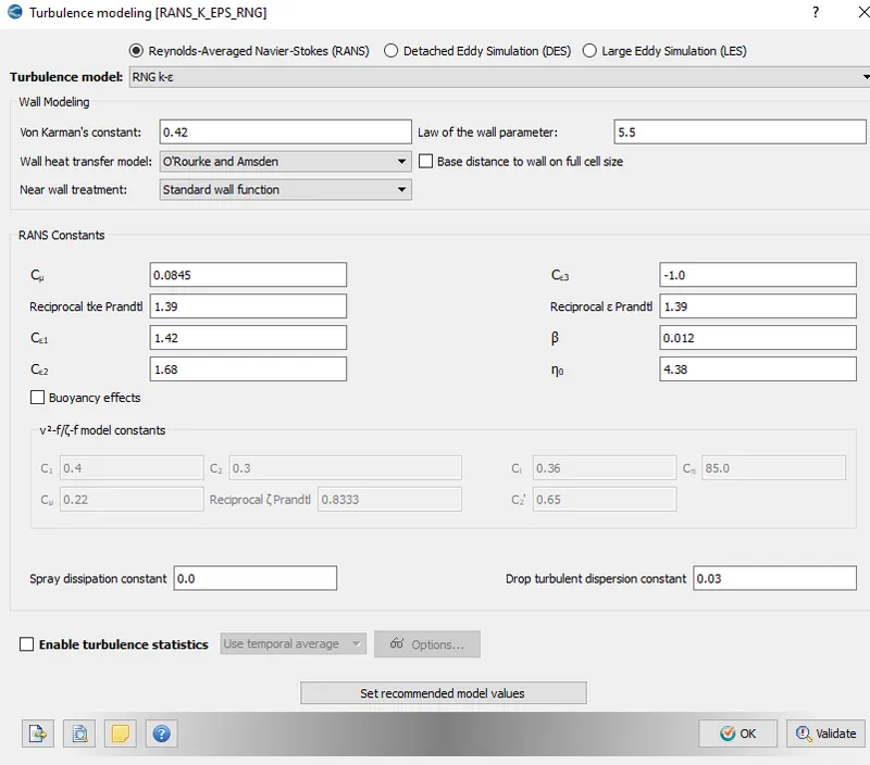
The turbulence is modeled by selecting the appropriate model in the turbulence option of the physical model. RNG k-epsilon with standard wall function is used for modelling the turbulence.
- Grid control:
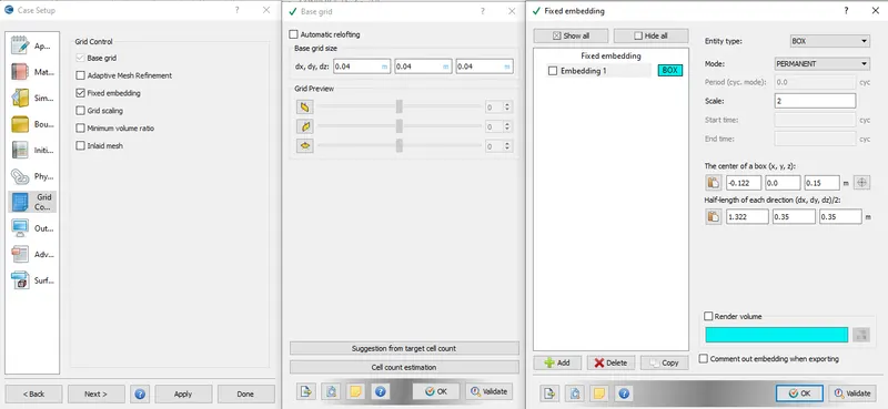
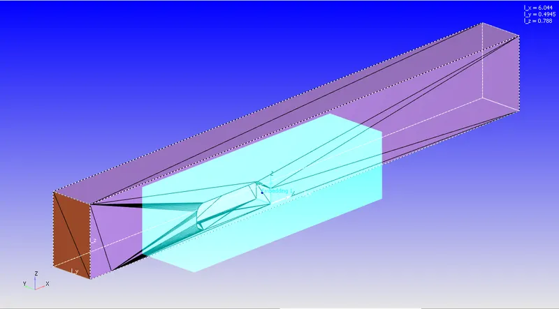
The base mesh size for the domain is defined in this tab as shown below. Along with it, box-type fixed embedding is used around the Ahmed body for refining the mesh surrounding it.
| Grid controls | Box type fixed embedding |
 |
 |
- Output and post-processing:
The flow variables of interest, which are to be post-processed after the solution are selected in this option, and also at how many intervals these are written to the output file. Also, wall output (BOUNDARIES ONLY) is enabled for the Ahmed body boundary zone to post-process the wall physics.
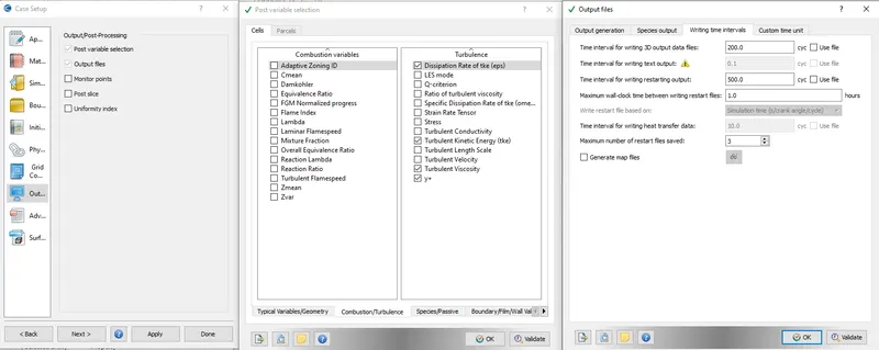
After all the above setup is completed final validation option is selected to check for the case setup is correct. After validation, the case setup files are exported using the export option in the File menu to the working folder. These files will be used by the CGYWIN terminal to run the solution.
VI. Solution in CYGWIN :
The solution is run in the CYGWIN terminal. First, we have to navigate to the respective working folder in the CYGWIN terminal, where case setup files are present. Then by executing the following command, the solution can be run:
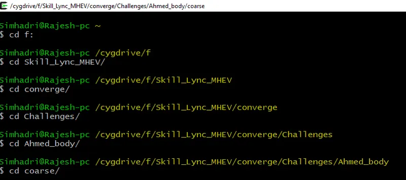
Running the solution:

The solution will run up to the total number of cycles or convergence criteria set in the run setup and the output files are saved to the respective folders.
VII. Post-Processing Results:
After the solution is complete, post-processing of the results is done using CONVERGE CFD and ParaView.
The plots are plotted in CONVERGE CFD, whereas to visualize the flow variables using contour plots the output files need to be converted to ParaView compatible files. This can be done in the CONVERGE CFD Post-Processing 3D tab.
Results Discussion:
1. Steady-state solution with coarse mesh:
A steady-state analysis with the coarse grid is run to check for the analysis setup faults. Also, the coarse mesh will aid in less computational time.
I. Grid:
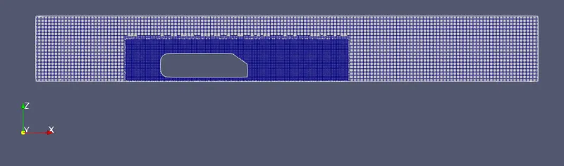
The above figure shows the coarse mesh used for the steady-state solution. Box embedding is used to refine the mesh around the Ahmed body surroundings.
II. Pressure and Velocity Contours:
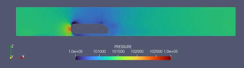
The below figures represent the steady-state Pressure and Velocity contours at the mid-plane (symmetry plane) around the Ahmed body.
| Pressure | Velocity |
 |
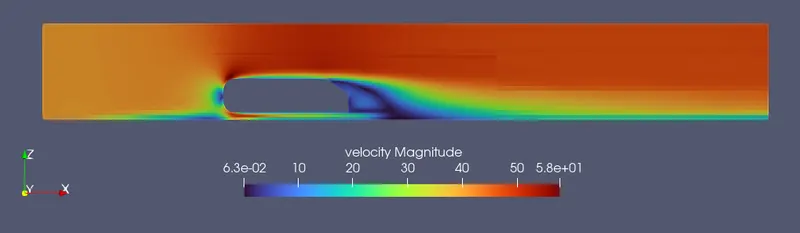 |
A high-pressure region is created in front of the Ahmed body due to flow stagnation, which in turn makes velocity. Also, a wake is formed behind the Ahmed body due to flow separation. The formation of wake leads to an increase in drag force on the body which in turn impacts the aerodynamic performance.
The following animations show the flow development around the Ahmed body.
| Velocity | Pressure |
Velocity variations with respect to height:
The variation of velocity with respect to height t different locations along the flow direction is plotted to compare the simulation results with experimental data [3]. The following plot compares the normalized velocity distribution around the Ahmed body between simulation and experimental results of [3].
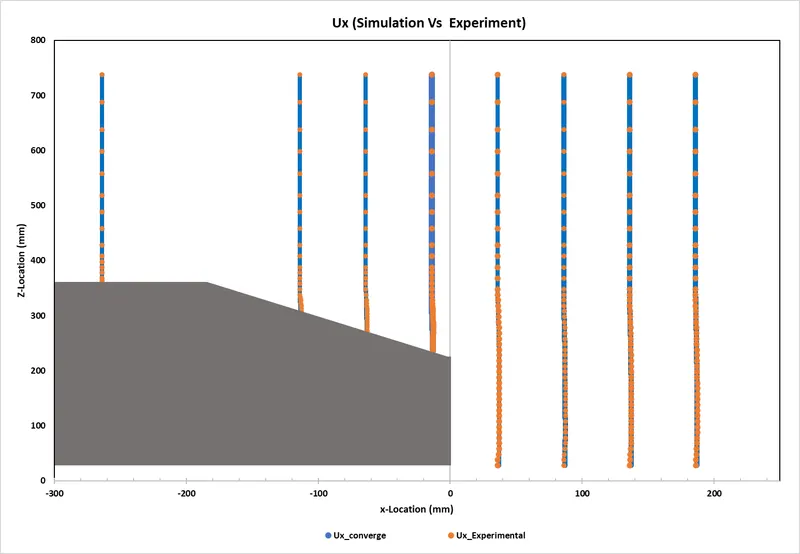
The above plot shows the normalized velocities with respect to location. More details about the plots and normalization can be found in the following attachment:
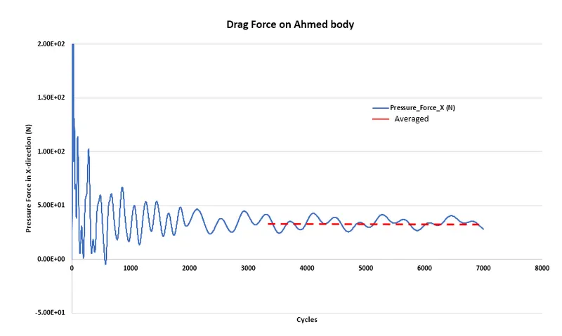
The above plot shows the Pressure force/Drag force (along x-direction) on the Ahmed body. It can be seen that after 3300 cycles the pressure force variation is almost repetitive. This is because of wake formation behind the Ahmed body. The average drag force on the Ahmed body is obtained by averaging the values between the 3300-7000 cycles result. The obtained average pressure force/drag force is given below:
Fd = 33.9 N
The above drag force computation and plot can be found in the above-attached line plots file.
The drag force can also be computed in Paraview, by selecting the frontal area of the Ahmed body and integrating the pressure force on the frontal surface. The obtained drag force from ParaView computation is given below:
Fd = 28.209 N
Further , computing the frontal area of the Ahmed body , the coefficient of drag is calculated as below:
Frontal area = A = 0.0243 m^2
Fd = 28.209 N
`C_d =F_d/(1/2rhoAV^2)`
`C_d = 28.209/(1/2*1.2*0.0243*40^2)`
Cd = 1.209
From the above discussion, it was observed that the pressure forces on the Ahmed body are having a repetitive phenomenon. Hence the flow over the Ahmed body is transient in nature. Also, due to computational limitations, a coarse mesh was used for the above analysis.
To have better accuracy and to capture the flow transient phenomenon, a transient analysis with refined mesh on a high-end computer can be carried out to achieve accurate results.
Conclusion:
A 3D steady-state numerical aerodynamic flow analysis over an Ahmed body prototype is performed in Converge CFD. The numerical results were compared with experimental data. Further drag force and coefficient of drag were also computed. Since the flow behind the Ahmed body has periodic flow pattern changes due to wake formation, a transient analysis would be suitable to accurately capture the flow physics. Refining the mesh will also lead to capturing the wall physics appropriately. Due to computational limitations, the analysis is performed with a coarse mesh.
References:
1. Ahmed, S., Ramm, G., and Faltin, G., "Some Salient Features Of The Time-Averaged Ground Vehicle Wake," SAE Technical Paper 840300, 1984.
2. https://www.comsol.com/blogs/studying-the-airflow-over-a-car-using-an-ahmed-body/
3. http://cfd.mace.manchester.ac.uk/ercoftac/doku.php?id=cases:case082