Week 10: Modeling and Simulation of flow around an Ahmed Body

Modeling and Simulation of flow around an Ahmed Body

• Aim:

Perform external flow simulation on Ahmed boddy and validate the results with experimental data. Design an Ahmed body with the wind tunnel using any CAD softwares and import the geometry onto converge and perform steady-state simulation with suitable turbulence model having the correct embedding settings and post process the results accurately to match the experimental data.

• Theory:

1. Ahmed body and its importance:

The Ahmed body is a generic car body (a simplified vehicle model). The airflow around the Ahmed body captures the essential flow features around an automobile and was first defined and characterized in the experimental work of Ahmed. Although it has a very simple shape, the Ahmed body allows us to capture characteristic features that are relevant to bodies in the automobile industry. This model is also used to describe the turbulent flow field around a car-like geometry. Once the numerical model is validated, it is used to design new models of the car.

Ahmed body is simplified car model created by Ahmed et in the 1980s to investigate the behaviour of newly developed turbulence models for complex geometry cases. The Ahmed body is made up of around front part, a movable slant plane placed in the rear of the body to study the separation phenomena at different angles, and a rectangular box, which connects the front and rear slant plane as shown. Ahmed body is a simplified model of a car body, but it demonstrates all the flow features involved in an actual case of a moving car. Current vehicle development needs a strong background in aerodynamics to improve flow control by means of active or passive control devices. The complexity involved in the automobile design especially due to the great number of accessories and devices that form its geometry makes the validation tasks unaffordable. The Ahmed model is a simple geometric body that retains the main flow features, especially the vortex wake flow where most part of the drag is
concentrated and it is a good candidate to be used as a benchmark test.

The Ahmed body represents a simplified, ground vehicle geometry of a bluff body type. Its shape is simple enough to allow for accurate flow simulation but retains some important practical features relevant to automobile bodies. Selection of the configuration of this body is governed by the requirement that it should generate the essential features of a real vehicle flow field except for the flow fields that occur due to rotating wheels, engine and passenger compartment, rough underside and surface projections. The model chosen would generate strong 3-D flows in front, relatively uniform flow in the middle and a large structured wake at the rear.

2. Reason for negative pressure in the wake region:

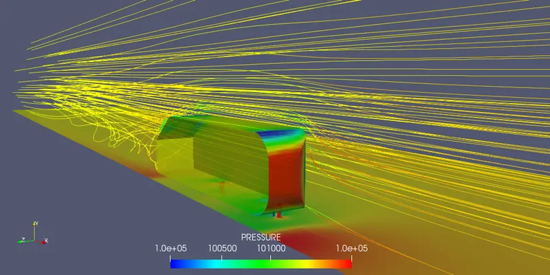
The path lines showing the exact circular motion or vorticity generation just at the rear end of the car. The separation takes two regions of distribution. One at the upper part of the rear and the other at the lower part of the rear end.

The path lines show about the nature of the fluid interaction with the rear end of the Ahmed body which here shows that the fluid just after leaving the contact from the slope still possess the momentum in it and the fluid particles near to the surface almost show the no-slip region which means the very least possible velocity of the fluid particles is in contact with the slope and base of the rear part. Thus the fluid particles away from the rear region having the higher pressure beside the wake region try to approach from the higher pressure region to the lower pressure region thus creating a circularity exactly in the wake region created.

The body penetrating the fluid creates a region of emptiness just beside its end due to the nature of the geometry of the body here which can be seen least in case of a perfectly streamlined shaped body. This emptiness created is a low-pressure region towards which the fluid column exactly behind the wake region which of atmospheric pressure tries to fill the space thus dragging the fluid column with it thus creating the region of vorticity. This also results in the huge pressure gradient in the region exactly rear of the body creating the –ve pressure at the end. Also, this is the layman’s reason why there is negative gauge pressure in the wake region.

3. Significance of the point of separation:

The fluid separation point can be defined as a point where the dv/dy i.e. gradient of velocity goes zero along with the dp/dx = 0, for the specific point. In more simplified term we can say that the point where the velocity gradient goes zero and the pressure gradient along the x- direction goes zero the point of separations starts occurring or the negative pressure gradient starts forming after that point. The point of separation cannot be understood just by single contour in hard and fast way. It can be supportively studied with the help of the dp/dx plots or velocity plots w.r.t the Y direction and other such plots in which we can see the nature of such physical properties like dp/dx=0, and dv/dy=0 experiencing in a particular region of fluid and body interaction.

4. Drag Coefficient:

The drag-coefficient quantifies the resistance of an object in a fluid environment. It is not an absolute constant for a body’s shape because it varies with the speed and direction of flow, object shape and size, and the density and viscosity of the fluid. The lower the drag coefficient of an object, the less aerodynamic or hydrodynamic drag occurs. In terms of a car, the lower the drag coefficient, the more efficient the car is. As well as affecting the top speed of a vehicle, the drag coefficient also affects the handling. Cars with a low drag coefficient are sought after, but decreasing the drag drastically can reduce the down force and lead to loss in road traction and a higher chance of car accidents.

• Procedure:

- Design of Ahmed Body using Fushion 360 CAD Software:

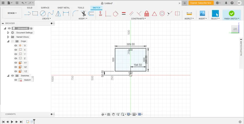
1. Create the Ahmed body 2D by starting at the back end of the car having square dimensions 389x288mm.

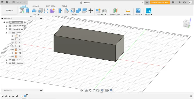
2. Extrude the Geometry along x direction having length 1044mm

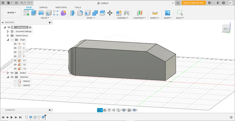
3. Give a fillet at the front of radius 100 with face select.

4. Create a triangle on the rear end and extrude to delete the excess to give a slant edge.

5. Now choose sketch on the bottom surface to add stilts, create a circle of dia 30mm and place the circle as per the dimensions provided.

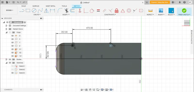
6. Create a construction line on the middle line of the plane and mirror the stilts on the other side.

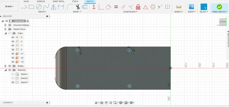
7. We have Completed the design of Ahmed body with slant angle 35 degrees

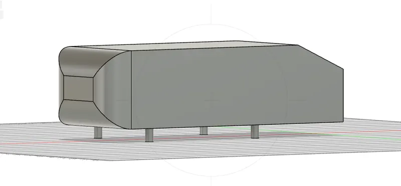
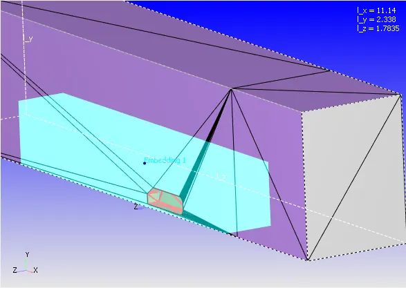
8. Create an Enclosure around the Ahmed body which is wind tunnel having dimensions, 3L in the front 5L in back and width of 2L, L is the length of ahmed body.

9. Since Ahmed body is having a symmetry geometry. Only one half can be used to save computational resources and also to have a finer mesh around the geometry. Which gives us accurate results and understanding good results.

- Boundary flagging and case setup:

1. After uploading the STL file containing the ahmed body with its enclosure. Boundary flagging is done before moving to the case setup.

2. The side and top walls can be set to symmetry BC. Bottom surface has to 2 sides, one with slip conditions at the inlet and no slip as the ahmed body approaches.

3. After flagging all the boundaries, transient state solver case setup is initialised.

- CALUCLATING THE DISTANCE FOR GROWTH OF BOUNDARY LAYER:

The condition statement given is that, the boundary layer should be 30mm thick at 400mm in front of the body. An approximation of boundary layer thickness over a flat plate is given by,

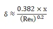
where `delta` is the boundary layer thickness (m), which is 30mm.

‘ x ’ is the length of the plate (m)

Re is the Reynolds number at location ‘x’

Here the unknown is

w.k.t Reynolds number,

Re=ρVL/µ

where `rho` is the density of fluid flow (air) which is 1.225 kg/m^3

V is the velocity of the flow, which is 40 m/s

`mu` is the dynamic viscosity of air, which is

but here instead of ‘L’ we have ‘x’ which is the length of the plate.

Hence,

Rex  =   ρVx/µ

Substituting in the above boundary layer equation, we get

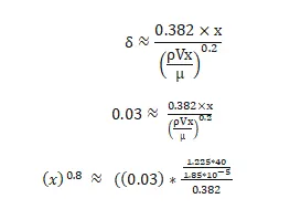
calculating for ‘x’ we get,

          (x)   ≈  1.66 m.

This means that at 1.66 m in front of the body there will be a boundary layer which is of thickness 30mm.

Hence to know the actual growth of boundary layer 400mm is to be added in front of the Ahmed body ie,,,

1.66 + 0.4 = 2.04 m.

Since we want a uniform velocity profile at the inlet where there should be no growth of boundary layer, let’s provide a boundary condition of ‘slip’ where the fluid motion is not zero and hence there will be no growth of boundary layer.

The slip distance is taken as one times the length of the body, ie,,,

1*1.044 = 1.044 m (slip distance)

Hence the inflow length from inlet to the front part of the body is 3.132 m ( ie,, 3*L).

Remaining distance is ‘Law of wall’ including Ahmed Body ( 6.264 m).

- Case setup:

1. Application type: time based

2. Materials:

a. Gas simulation: air

b. Global transport properties: Deafult

c. Species: O2 and N2

3. Simulation parameters:

a. Run parameters:

Transient solver, full hydrodynamic, compressible

b. Simulation time parameters:

- End time- 1 sec

Calculating end time:

End time is calculated by analysing the flow time from the inlet to outlet and the inlet velocity at which the flow generates, by knowing these 2 parameters, we can calculate the end time.

Since, length of the pipe is approx 11.24m and velocity at inlet = 40 m/s

Therefore, end time = distance of pipe/ inlet velocity

Which implies, 11.14/40= 0.2785 sec

It takes 0.2785 secs for the flow to complete 1 cycle, we can have 4 cycles which is 4x0.2785= 1.114 `~=`1 sec

- Time step- 1e-6

- min time step- 1e-6

- max time step- 1

- Convection CFL number- 0.5

c. Solver Parameters-

- Solver type- density based solver

4. Boundary Conditions-

a. Inlet- Inflow

- Total pressure- NE

- Inlet velocity- 40m/s

- Initial temp- 300K

- Species boundary condition- add air

b. Outlet- Outflow

- Pressure- NE

- Backflow - temp= 300k

- add air

c. No-Slip bottom surface - Wall, no-slip BC

no slip condition- The contact region between wall surface and fluid region tends to create high friction and create a 0 velocity of fluid flow, and due to viscosity of fluid, the fluid layers tend to undergo shear stress and have high pressure and overlap on eachother which eventually forms a fully developed region where velocity is max and constant and having low pressure.

d. Slip bottom surface- Wall

- Slip BC

e. Wall Symmetry(sides and top)- Symmetry BC

- Symmetry

f. Ahmed body- Wall

- Law of the wall

- Omega wall conditions: Wall model

5. Initial Conditions and Events:-

- Regions and Initialization:

x-velocity: 40m/s

Pressure- 1.5e5 Pa

Temperature: 300K

Add- air

6. Physical Models:-

- RANS k-w SST

7. Grid Control:-

a. Base Grid:

dx = 2e-4m, dy = 2e-4m, dz = 2e-4m

b. Embedding:

- Box embedding:

- Boundary type: Ahmed Body, permanent mode embedding.

Scale- 3

Number of layers- 6

Embedding is the means by which we can refine the mesh to a value that is lower than the prevalent base size. This is especially useful if we are looking to refine near wall to capture the boundary layer or the wake of a body more accurately.

8. Post-Processing:-

- Post Variable Selection:

Select the parameters needed to be post processed.

- Output files:

- Enable Boundaries only under wall output in output generation,this helps us to get averaged values of certain physical quantities.

We need to set a time interval for the files to be saved during each set of iterations. It is best suited to have a min of 100 saved files for every simulation. Therefore we need to calculate the time interval for writing the output files based on our end time given in run parameters.

Restart files help in restoring the files if there is a sudden power cut/ crash which is not helpful or might end up loosing the entire data, therefore the restart files helps in resuming the simulation form the point we lost contact. Restart files time interval can be same as the writing files interval which is safe and healthy.

In this case- since the end time is 1, we can have a time interval of 0.01 and the total files created will be 100.

• Results:

- Mesh:

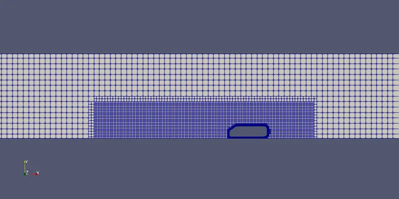
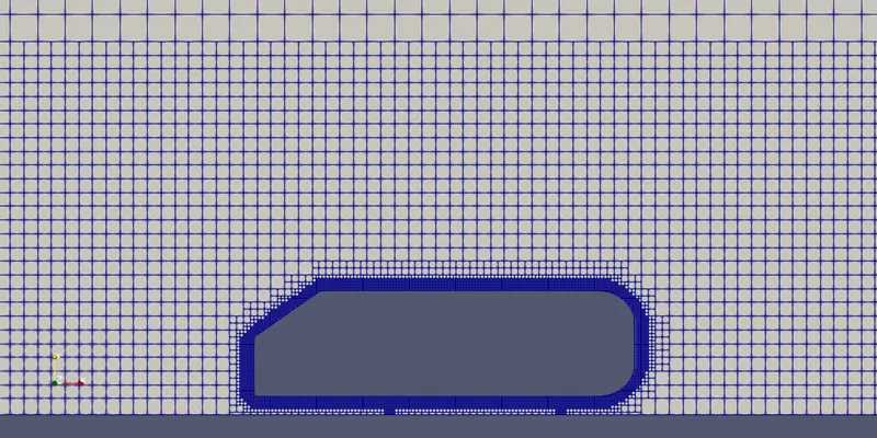
Base mesh grid of 0.15m was implemented for the entire geometry, box embedding is used as a second enclosure, to capture accurate results around the car geometry. Box embedding scale of 2 and boundar layer embedding of Ahmed body was used to have a very fine mesh at the boundary to capture the boundary layer physics and accurate flow separation at the rear end. Scale of 5 and number of layers 6 was implemented.

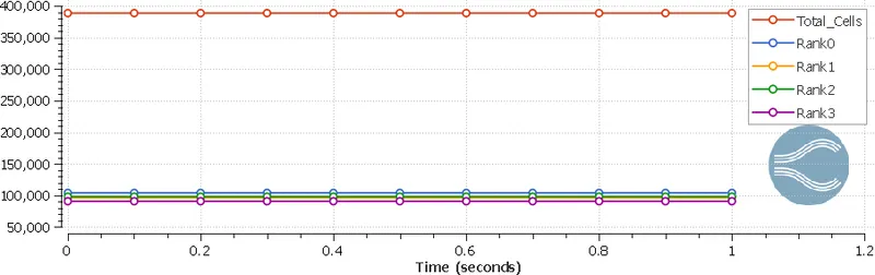
- cell count:

- Drag Coefficient:

Drag Coefficient is Calculated using the data collected from the drag force plot. Using the average pressure in x-direction(i.e drag force), we can use the value to calculate Cd.

-Drag force:

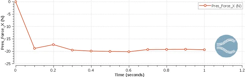
Above plot shows the drag force generated on a body when the body moves through a fluid at 40 m/s ( although the science of body moving over a stationary fluid or fluid moving over a stationary body remains the same).

At the end of the simulation the drag force generated on the body converges to be 52.2 N.

Therefore we have,

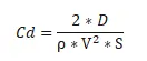
D is the drag force in Newton (N)

is the density of the fluid or continuum

V is the free-stream or relative stream velocity

S is the surface area

Here ‘S’ can be calculated to be frontal cross-sectional area ie,, we have length as 288mm and breadth as 389mm so the area of the body turns out to be

= 0.288*0.389

= 0.112 m^2

We know density of air at 300K, which is 1.225 kg/m^3

We also have velocity, V = 40m/s.

Therefore,

Cd = 2x 19.40/ 1.225x 0.253x (40^2)

Cd= 0.078 (for Half Ahmed body)

Which implies for full Ahmed body,

Cd= 0.156

- Lift coefficient:

Lift Coefficient is calculated using the data collected from the Lift force plot. Using the average pressure in y-direction(i.e lift force), we can use the value to calculate Ld.

- Lift force:

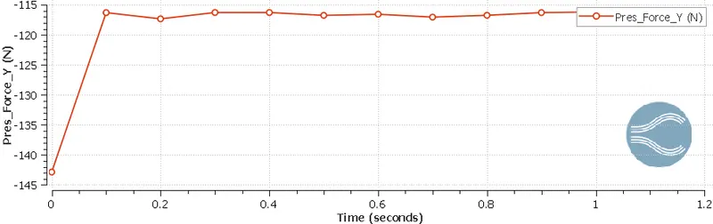
Above plot shows the lift force generated on a body when the body moves through a fluid at 40 m/s (here in our case vertical direction is ‘Y’ axis).

At the end of the simulation the lift force generated on the body converges to be 116.184 N.

Therefore we have,

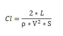
‘L’ is the Lift force in Newton (N)

`rho` is the density of the fluid or continuum

V is the free-stream or relative stream velocity

S is the surface area

Hence,

Ld = 2x 116.184/ 1.225x 0.253x (40^2)

Ld= 0.468 (for Half Ahmed body)

Which implies for full Ahmed body,

Ld= 0.937

- Velocity:

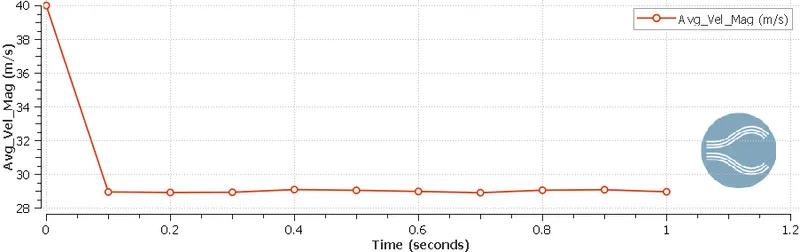
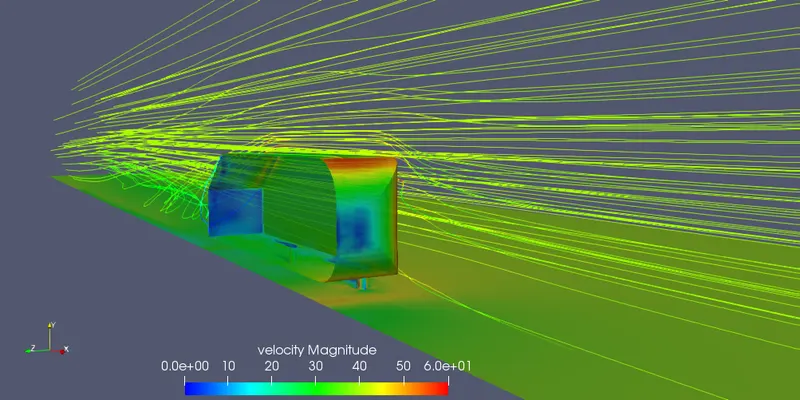
Above plot shows the variation of velocity with time. Initially the flow has a velocity of 40 m/s and once the flow encounters the Ahmed Body the velocity decreases in the front portion of the body. Once the simulation reaches the steady state, velocity achieved is 25 m/s.

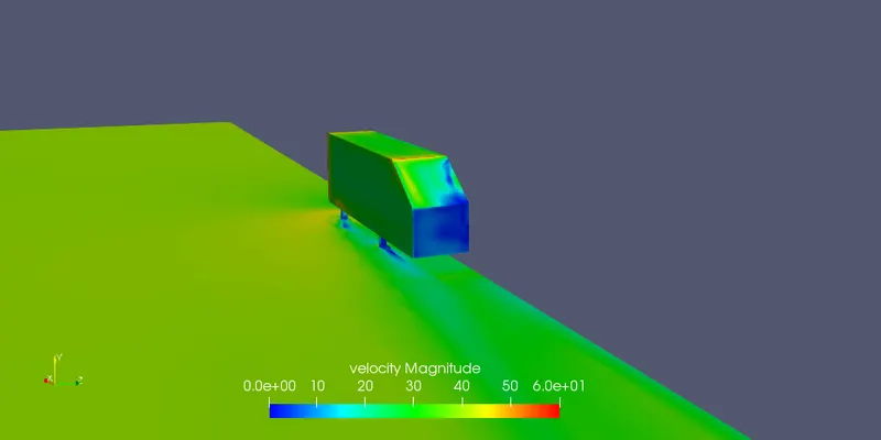
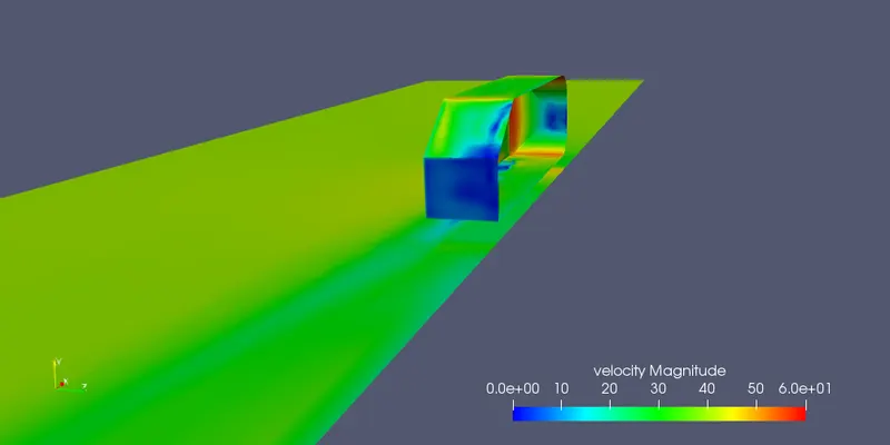
- Velocity contours:

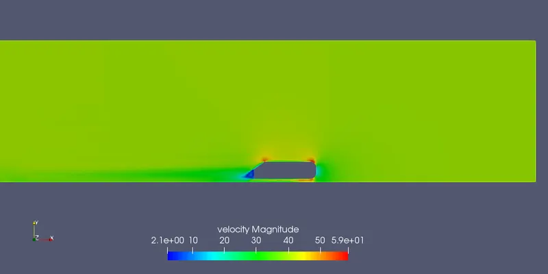
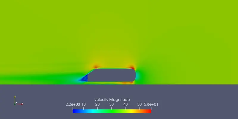
a. Velocity slice contour:

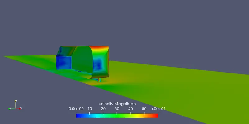
b. Velocity block contour:

- Velocity Streamline:

- Velocity Animation:

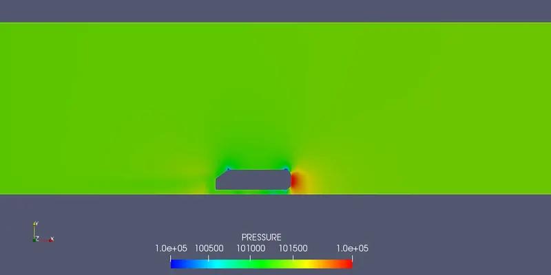
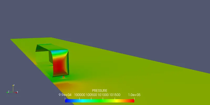
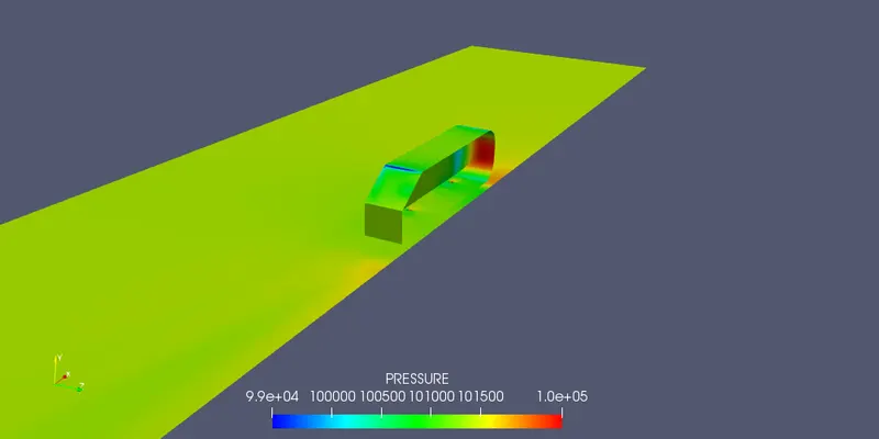
- Pressure:

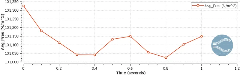
Above plot shows the variation of pressure with time. To understand it better, there are some of the contours of pressure distribution over the body, shown below.

- Pressure slice contours:

- Pressure block contour:

- Pressure streamline:

- Pressure animation:

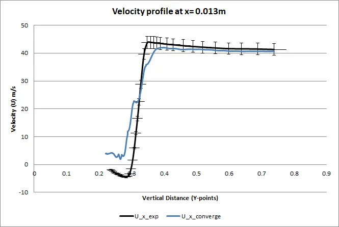
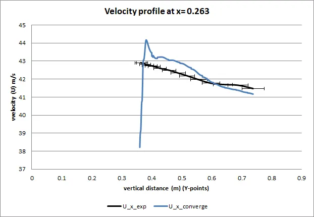
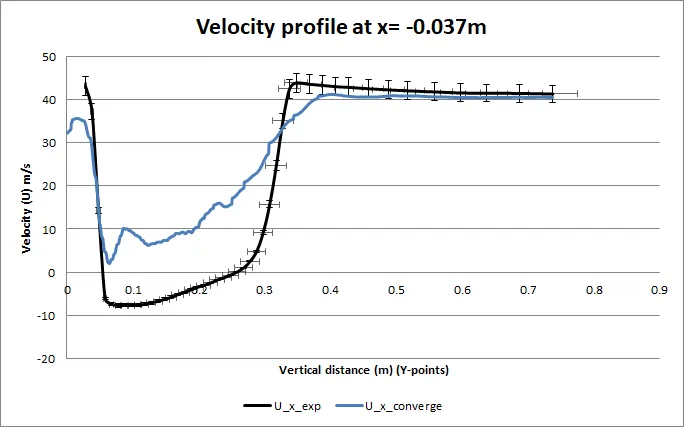
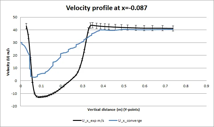
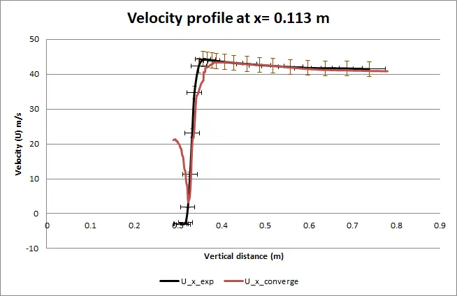
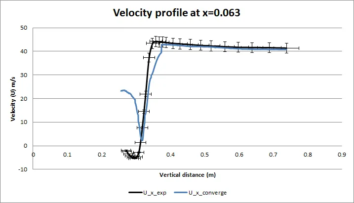
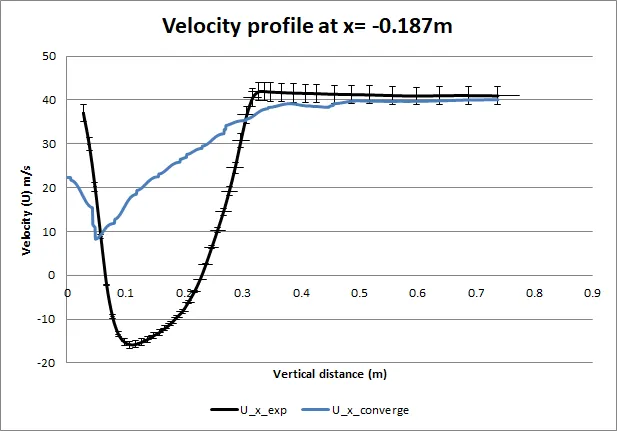
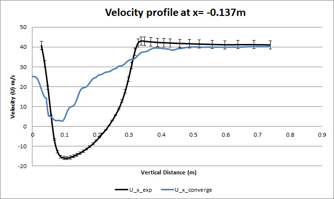
- Comparision of simulation results with Experimental data using line probes at different locations of X:

The origin of the simulation geometry is located exactly as the experimental setup, but the velocity is flowing in negative x-direction therefore the line probes location are opposite in signs to that of experimental line probes.

1. At x= 0.013m

2. At x= 0.263m

3. At x= -0.037m

4. At x= -0.087m

5. At x=0.113

6. At x= 0.063m

7. At x= -0.187m

8. At x= -0.137m

• Conclusions:

- The total drag coefficient of the Ahmed body is the key measurement for this simulation.

- It is made up of measurements for the pressure coefficients in the front, slant, and base of the body as well as the body’s skin friction.

- In the results of our simulation, the total drag is very well predicted but the individual measurements deviate from the experimental results in varying amounts. For a slant angle of 35-degree the value of drag and lift coefficients are found to be 0.156 and 0.937

- When the body is moving at 40 m/s (although the science of air moving around stationary body or body moving around the stationary air is same) it encounters a resistive foroce of 38.8 N ie,, the drag force.

- Even better simulation results can be achieved with increase computational power and decrease in grid size.

- The plots show that the simulation results are coinciding with some parts of the plot which indicates that out simulation is performed correctly.

- To decrease the Drag, we can decrease our slant angles therefore reduced flow separation is achieved at the rear end of the car. Which gives us better performance efficiency of the vehicle.