Week 10: Modeling and Simulation of flow around an Ahmed Body
Aim:
Model and Simulate flow around an Ahmed Body using Converge CFD and compare the simulation results with provided experimental data.
Objective:
- Create the CAD model using any CAD package.
- Setup a Coarse CFD simulation
- Setup the virtual wind tunnel
- Apply the right boundary conditions and solver settings
- Show an animation of the velocity distribution, pressure distribution on a cut plane.
- Enable wall-averaged outputs to measure the drag and lift forces.
Introduction and Theory:
Ahmed reference model is a generic simplified car geometry that can be used to investigate
main flow features in the wake of the ground vehicles. The angle of the rear slanted surface strongly influences the flow downstream of the Ahmed body, which indicates that the development of three-dimensional vortex separation from the rear slant surface produces a major component of the aerodynamic drag acting on the vehicle. Ahmed et al. were the first to study 3-D external flow analysis on the Ahmed body.
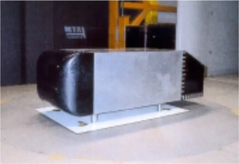
The Ahmed body is made up of around the front part, a movable slant plane placed in the rear of the body to study the separation phenomena at 25`overset@`, 35`overset@`, and a rectangular box, which connects the front and rear slant plane. The most significant feature of the body is the 25`overset@`, 35`overset@` angle of the rear slant. Air is used as a working fluid. The inlet velocity of the fluid is 40 m/s.
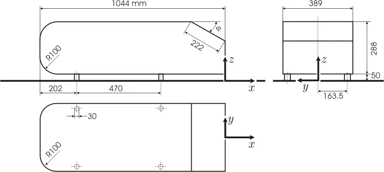
The geometrical shape of the Ahmed body (simplified car body) investigated is depicted in Figure. Due to the considerable deviation of its geometry from normal vehicles, the body represents the basic aerodynamic properties of a vehicle, especially in the rear part. The rear slant angle ϕ has a strong effect on the aerodynamic drag and lift at the back.
Both the drag and lift coefficients change abruptly at the angle ϕ=30°. Therefore, this angle is called the critical slant angle.
Case Setup:
1. Using the Ahmed Body Drawing mentioned above, a 3D model is created. The slant angle for Ahmed body is assumed to be `varphi` = 35`overset@`
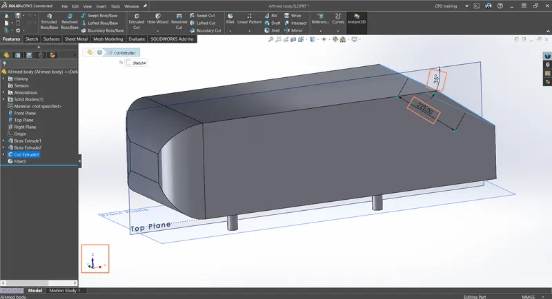
2. This 3D model is saved as .STL file and later imported into CONVERGE Studio Software.
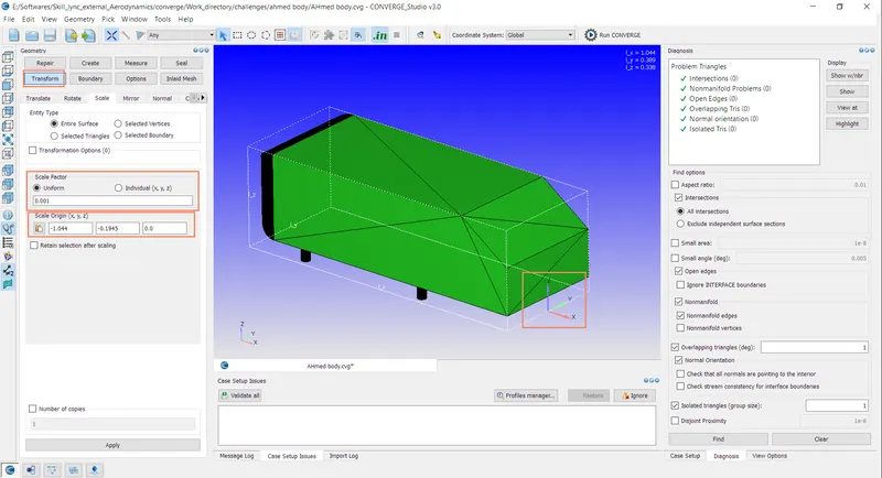
3. The only Ahmed Body geometry imported in the CONVERGE Studio, but virtual wind tunnel is created for well-calculated and well-defined tunnel dimensions. For this, the following calculations are done to imply constraints to the bounding box.
- Given Data: Boundary Layer Thickness is 30 mm at 400 mm in front of the Ahmed body.
- Boundary layer thickness on a flat plate:
- `delta~~ (0.382 * x) / (Reundersetx^(1/5))`,where,`delta` = boundary layer thickness in `m`,`x` = length of the plate in `m` `Reundersetx`= Reynolds number at location `x`
- Here,
- `delta`= 0.03 `m`0.03 =`(0.382*x)/((rho*v*x)/mu)^(1/5)`
- As we know,`v`= 40 `m/s`
- At 300 K temperature, for air, `rho`= 1.177 `(kg)/(m.s)`, `mu`= 1.846 x 10^-5
- `:.` `x`= 1.25 `m`
- Boundary layer thickness on a flat plate:
- Thus, the above-calculated value is the length at which the boundary layer thickness reaches 30 mm. So the actual length in front of the Ahmed body can be calculated as follow.
- 0.5 m = Assumption for free slip region. This free slip region avoids the boundary layer formation.
- 0.5 + 1.25 + 0.4 = 2.15 m
- In order to calculate and register the turbulence/wake formation on the leeward side, the length of the wind tunnel is taken as 5 to 10 times the length of the Ahmed body. Considering 5 times the length of the Ahmed body.
- Total length = 2.15 + 5*1.25 = 8.414 m
- The height and width of the wind tunnel are taken as 2 times the length of the Ahmed body in order to facilitate the 3D flow to happen in the way it should. This is done in order to avoid the top and side walls obstructing the flow of the fluid.
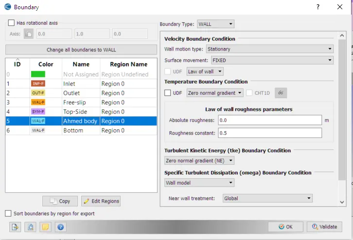
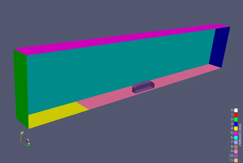
4. Then, the boundaries are flagged accordingly, such as the inlet, outlet, top and sidewalls, Free-slip wall, the law of the wall region, and the Ahmed body.
| Inlet | Inflow boundary: Velocity along x-dir= 40m/s and fluid medium air is added. Pressure-Neumann BC. |
| Outlet | Outflow boundary: Pressure=1atm(101325Pa) and fluid medium air is added. Velocity-Neumann BC |
| Free-slip Region | Wall boundary: Slip-wall option is selected as the boundary layer formation is not required in this region. |
| Law-of-the wall region | Wall boundary: Law-of-the-wall option is selected as the boundary layer formation is required in this region. |
| Top and side Walls | Symmetric boundary: As the boundary layer formation is not required in the top and sidewalls, this BC is given. |
| Ahmed Body | Wall boundary: Law-of-the-wall option is selected as the boundary layer formation is required in this region. |
5. The input conditions are given by means of setting the case set-up:
- The material/ fluid medium is selected as air and various other properties of the fluid are set to their default values.
- Then the simulation parameters are set as follows:
a. The transient simulation option is selected under the Run parameters as it is a time-dependent simulation.
b. The time for simulation is found based on the flow-through time. The flow thro' time is calculated as follows:- Flow-through time = Length of the wind tunnel / Velocity of fluid
- As calculated, the length of the wind tunnel = 8.414 m
- Velocity of fluid = 40 m/s
- Thus, flow-through time = 8.414 / 40 = 0.21035 sec.
- Generally, the time for simulation is 3 to 4 times that of the Flow-through time; here approximately 3 times, i.e.,
- Time for simulation = 3 x Flow-through Time = 3 * 0.21035 = 0.63105 sec `~~`0.65 sec.
- This time is given under the Simulation time parameters
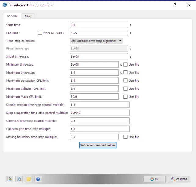
- Flow-through time = Length of the wind tunnel / Velocity of fluid
- The density-based solver is selected under Solver parameters. The initial values for the simulation, such as the velocity is set to 40m/s and a region is defined with air as a fluid medium.
- The `k-omega` turbulence model is selected under the Physical models. This model is a combination of RNG `k-epsilon`turbulence model and Standard `k-omega`model. This acts as `k-omega`model near the wall boundaries and RNG model away from the wall. Hence, it gives an accurate prediction of the simulation both near a wall and away. Moreover, it is accorded for its automatic wall treatment.
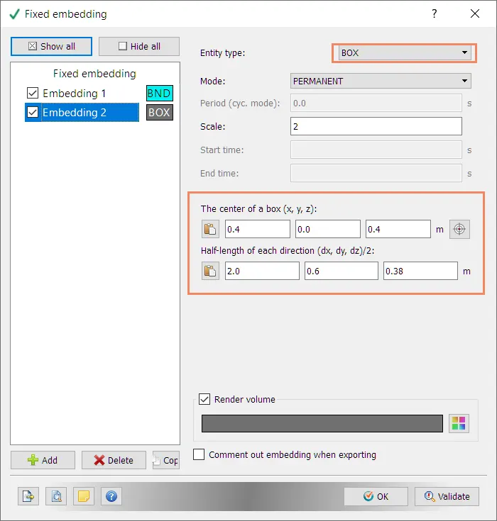
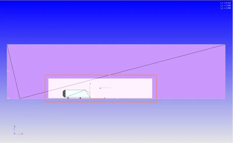
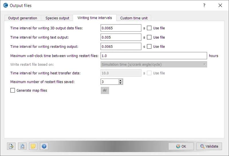
6. After setting up the grid size and embedding scale, the input files are generated and exported to a folder. Using Cygwin, the converge executable files are run and output files are generated.
7. These outputs are converted into a form Paraview can interpret, by means of the option available in converge studio to run the post-convert executable.
8. Then the outputs are post-processed using Paraview software and the simulation results are analyzed.
(The simulation is run with a higher degree of refinement in a system with higher capacity once the coarse simulation results are found valid. This simulation is run with half Ahmed body(i.e., Ahmed body is cut into 2 symmetric halves) to reduce the number of cells, which does not affect the simulation results in any way. So, the results of this simulation are also included in the below section along with the coarse simulation results)
Results:
Setup in block colors:
Velocity Contour:
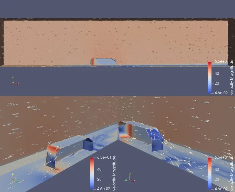
The flow is diverted to a greater extent by the front surface as its corners are rounded(i.e. filleted to a higher radius)
The nature of flow on the leeward side is due to the wake formation, which is due to the flow separation and recirculation.
The flow separation is accorded to the geometry of the Ahmed body, i.e., the slant angle.
The velocity is very low on the windward side because the airstrikes the front part and loses its kinetic energy.
Unlike the above case, the velocity is low on the leeward side due to the flow separation taking place at that location, which causes flow-reversal or recirculation. Due to this, a partial vacuum is created, thus leading to low velocity in this region.
The velocity is higher in the top and bottom part of the body because of the deflected air, due to its encounter with the body flows over the top and bottom surface. This adds up to the flow of air already existing in this location.
Velocity Animation of flow over Ahmed's body's velocity body. The higher velocity in the top-rear edge denotes the arrival of the point of flow separation. Due to this fact, the velocity is higher (Note: The velocity is higher just at the point which is in proximity to the point of flow separation and not in the region of flow separation!)
The low-velocity region(as explained earlier) along the trailing edge is called the wake region, which is due to the slant angle of the Ahmed body(35deg), i.e. it is accorded to the geometry.
This seems to move because of the nature of the vortices formed in the region due to the recirculation of air. This contributes to the majority of the drag force
on the body as it causes suction to take place in this location(i.e., a negative pressure) which ultimately adds up to the drag on the body.
Pressure Contour:
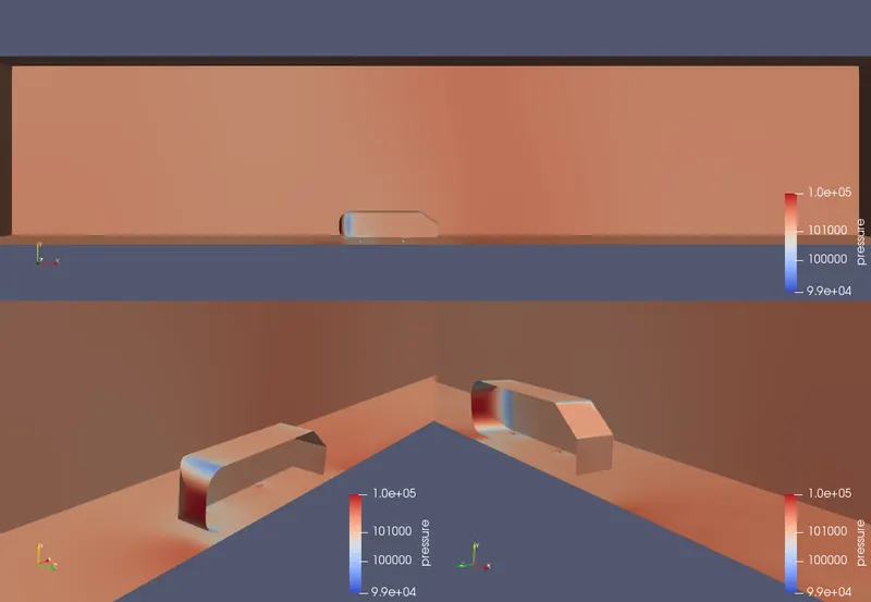
As the airstrikes the front surface, the kinetic energy is converted into pressure energy, which leads to the drastic increase in pressure in this area, this pressure is known as stagnation pressure as the fluid stagnates here. Even this contributes to some amount of drag.
The lower pressure in the top & bottom sides and the top-rear edge are accorded to the high velocity in these regions. As the velocity increases the pressure decreases.
Drag Force Vs Time plot:
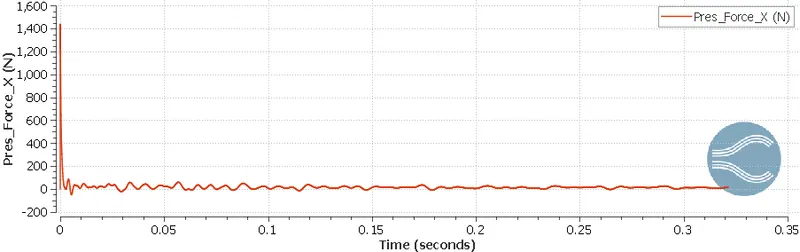
- The drag force (Pressure Force X) has attained a steady state.
- The drag force converges to a value of about 12.12528072 N.
- Now using the formula to calculate the Coefficient of drag,
- `Fundersetd`= `1/2.Cundersetd*rho*A*v^2`
- Here, `Fundersetd`= 12.12528072 N , `rho` = 1.177 kg/m^3, A = Frontal Area = 0.288 x 0.398 = 0.112 m^2 , `v`= 40 m/s
- `:.` `Cundersetd` = 0.1149760.
Lift Force Vs Time Plot
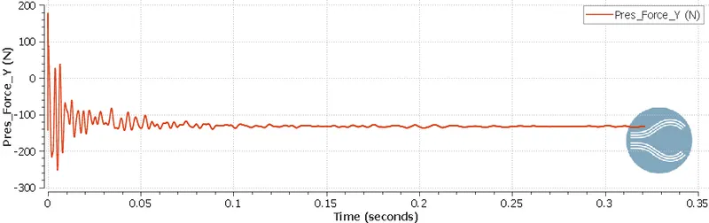
- The Lift force (Pressure Force Y) has attained a steady state.
- The Lift force converges to a value of about -132.842 N.
- Now using the formula to calculate the Coefficient of Lift,
- `Fundersetl`= `1/2.Cundersetl*rho*A*v^2`
- Here, `Fundersetl`= -132.842 N , `rho` = 1.177 kg/m^3, A = Frontal Area = 0.288 x 0.398 = 0.112 m^2 , `v`= 40 m/s
- `:.` `Cundersetl` = -1.2596530.
Drag Co-efficient calculated using Paraview:
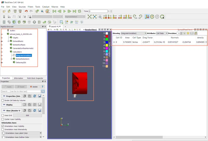
| Frontal Area | Drag Force | Velocity:0 | Y-plus |
| 0.765693 | -2.65477 | 18.6559 | 83.8225 |
Comparison of Velocity along x and y-coordinate with :
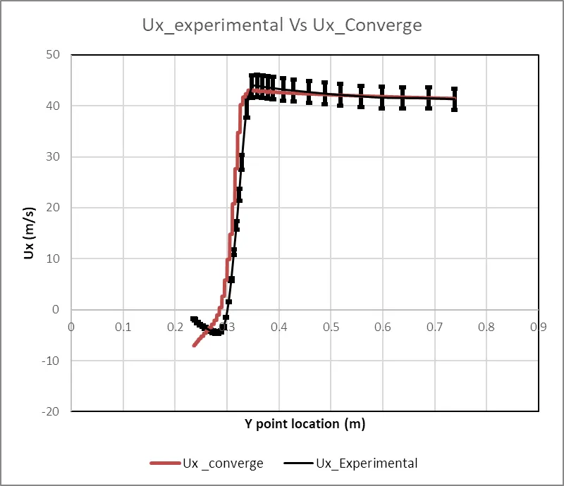
After the simulation has run, it is post-processed using Paraview software. In Paraview, the plot over the line the feature is used to plot the required variable along a line, whose endpoints are specified. Here, the velocity along the x-direction is plotted w.r.t. the Y-position, for that the lines are drawn as shown below.
These are drawn one by one, at stated locations, using the plot over line tool and the data is extracted and saved in an
Excel
file. Then the experimental data provided is compared with it by plotting. (Note: The origin stated in the below figure(the experimental origin) and the origin of the wind tunnel are different so, in order to plot the lines at the exact locations as that of experimental data, the points are mapped from the experimental origin to the wind tunnel origin by adding the difference between x-coordinates of the origins, here 3.1095m to the corresponding x-coordinates as the origins are collinear here).
|
x= -13 mm |
 |
| x = -263 mm | 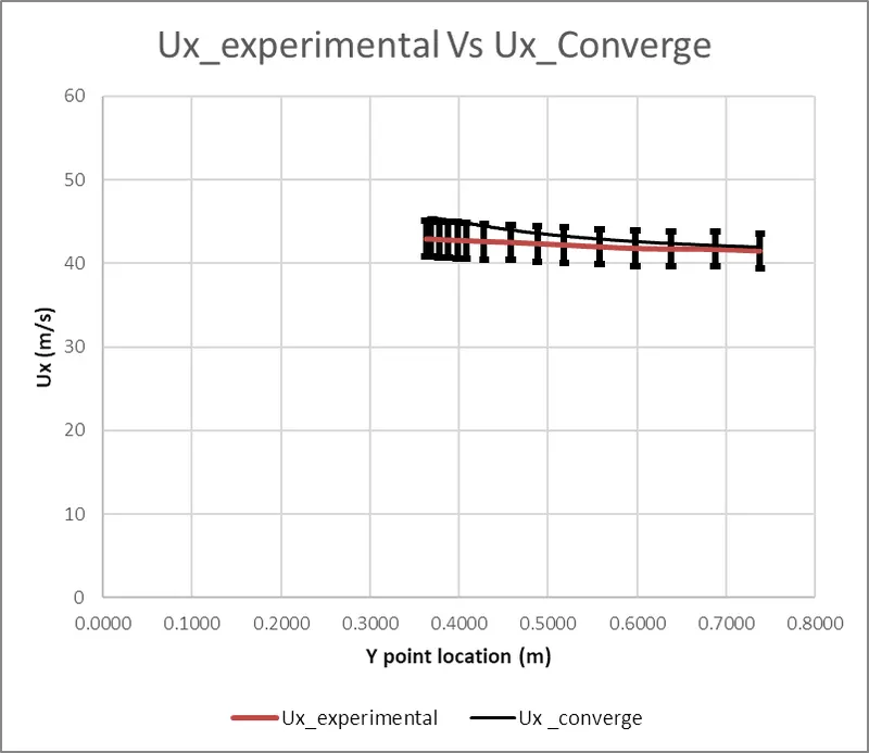 |
| x = 37 mm | 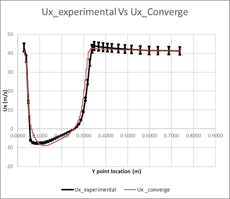 |
| x = 87 mm | 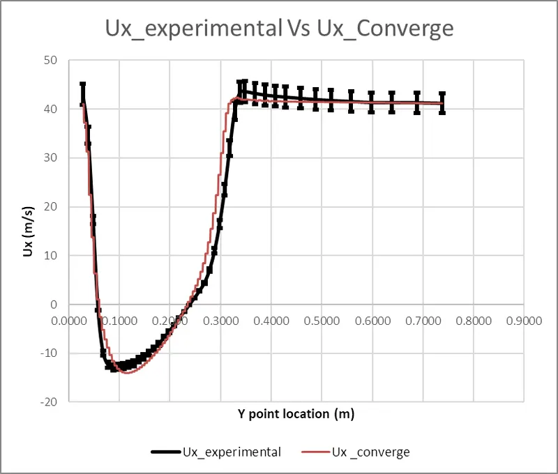 |
| x = -113 mm | 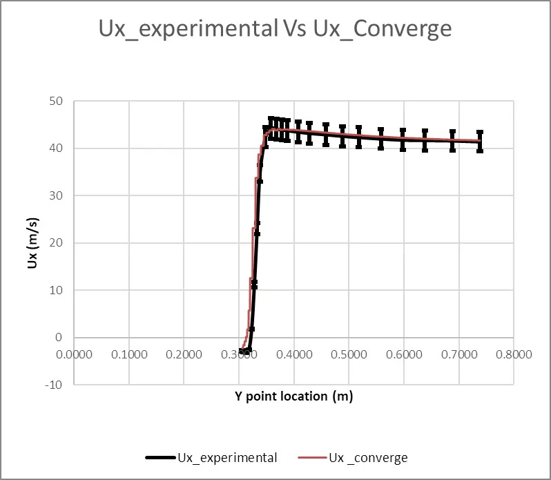 |
| x = -63 mm | 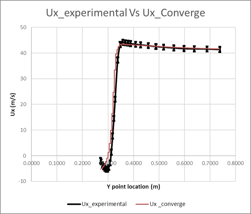 |
| x = 187 mm | 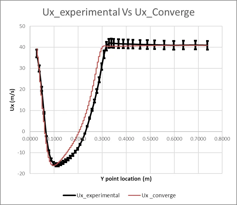 |
| x = 137 mm | 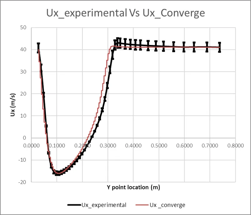 |
Normalised Velocity Plot:
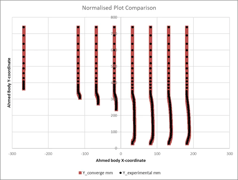
Normalization is done to visualize the velocity profile and compare it a bit easier. In order to normalize, for each line probe (both experimental and simulation data), the velocity at each point in the line probe is divided by the maximum velocity along the line and multiplied by an amplification factor, here 5. Then this value is subtracted from the x-coordinate value of the line so that it could be plotted for comparison. The below plot shows the normalized velocity plot, which suggests that the simulation and experimental data coincide to a greater extent. This shows that the simulation is valid. (Note: For verification, the results of a simulation run in a high configuration system have been included in the last)
Summary of Results:
1. From the graphs, we can see that the probes at the negative location are matching well with the experimental data compared to the probes on the positive side.
2. On the positive side, we can see that the error percentage in the graphs is greater than 5%. This is because of the grid size. We can reduce the grid size or simulate only one symmetric half with a reduced grid size.
3. The error on the positive side is greater because of the Drag produced on the rear side of the body. The rear side is positive from origin.
4. To capture this wake region correctly a smaller grid size and greater computational power are required.
5. From the Velocity contour, it is observed that after passing through the geometry there is a region where recirculation happens this region is called as wake region. Due to this low pressure, the air at the front tries to come back which increases the drag. The air after exiting the cylindrical pillars forms vortices. These vortices can be observed from the top view.
6. It is also observed that the lift obtained is negative which means that it is downward force. This force helps racing cars to stay on the ground. But for alow-efficiency vehicles such as a truck, this force is not desirable. Hence the shape of the truck/trailer will be optimized to reduce the negative lift
Conclusion:
- The flow over the Ahmed Body is simulated and aerodynamics-related parameters were calculated and obtained.
- The major amount of drag is produced by the rear part of Ahmed body's where the wake region is created.
- A comparative study with experimental data has been performed.