Week 10: Modeling and Simulation of flow around an Ahmed Body
MODELING AND SIMULATION OF FLOW AROUND AN AHMED BODY
Aim:-
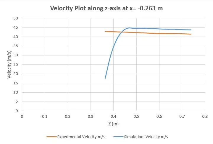
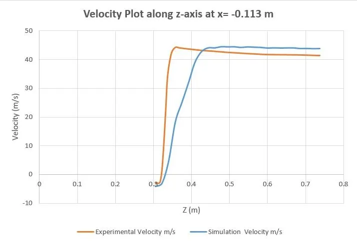
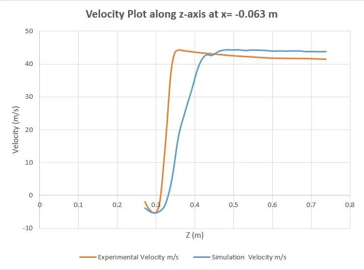
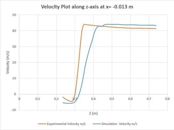
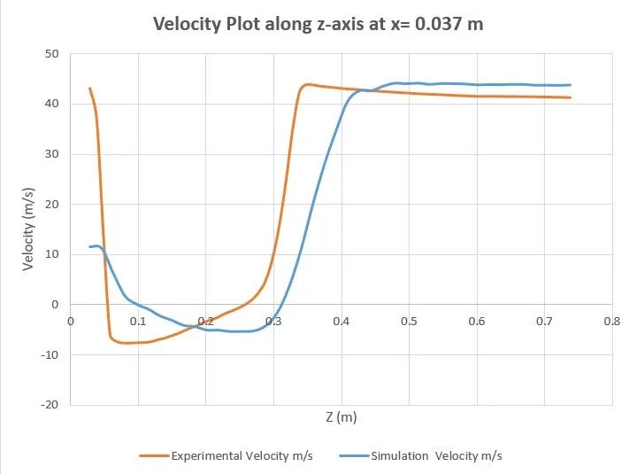
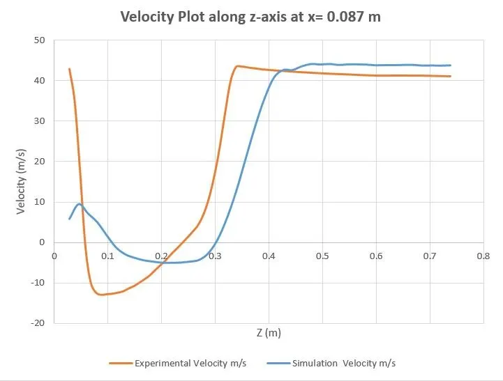
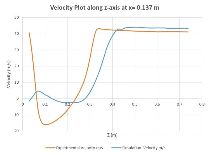
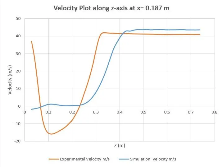
To modeling and simulate the flow around the Ahmed body and calculate drag force using ParaView. Plot the velocity line probes at different x locations along the z-axis and validate the experimental data and simulation data.
Objective:-
- Create the CAD model of Ahmed body using any CAD packages.
- Setup coarse CFD simulation.
- Create the virtual wind tunnel with appropriate dimensions.
- Apply right boundary conditions and solver settings.
- Calculate drag force and drag coefficient using ParaView.
- Plot velocity at different x locations using line probes.
- Compare the experimental data and simulation data.
Theory:-
Ahmed body:-
The Ahmed body is a generic car body. The airflow around the Ahmed body captures the essential flow features around an automobile and was first defined and characterized in the experimental work of Ahmed body. Although it has a very simple shape, Ahmed bod allows us to capture characteristic features that are relevant to bodies in the automobile industry.
This model is also used to describe the turbulent flow field around a car-like geometry. Once the numeric model is validated, it is used to design new models of the car.
Calculations:-
1. Reynolds number:-
`Re = (uxxL)/(nu)`
where,
`u = "Velocity of the Air" => 40m//s`
`L = "Height of the ahmed body" => 0.288m`
`nu = "Kinematic viscosity of the air" => 15 xx 10^6 (m^2//s)`
`Re = (40 xx 0.288)/(0.000015)`
`color(red)(Re = 768,000)`
2. Boundary layer thickness (`delta`):-
[Note:- 30mm thick at 400mm in front of the body]
`delta = (0.382*x)/(Re)^(1/5)`
where,
`delta = "Boundary layer Thickness" =>0.03m`
`Re = "Reynolds Number" => 768,000`
`x = "Distance from the boundary layer"`
`x = (delta*Re^(1/5))/0.382`
`x = (0.03xx (768000)^(1/5))/(0.382`
`color(red)(x = 1.1806 m`
3. Virtual Wind tunnel Dimension:-
- x = 10.88 m
- y = 1.8 m
- z = 1.389 m.
In x-axis 2 m (Slip region), 1.18m + 0.4m (30mm thick at 400mm in front of the Ahmed body), 1.044m (Ahmed body length), 6.264m (6x length of the Ahmed body).
X = 2m+1.18m+0.4m+1.044m+6.264m = 10.888m.
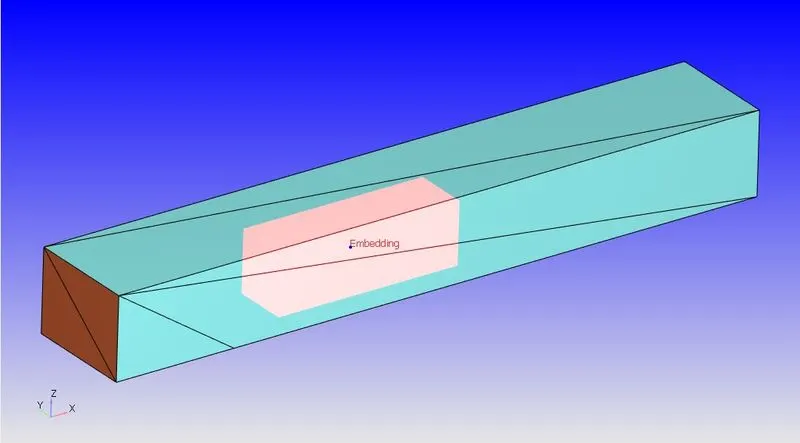
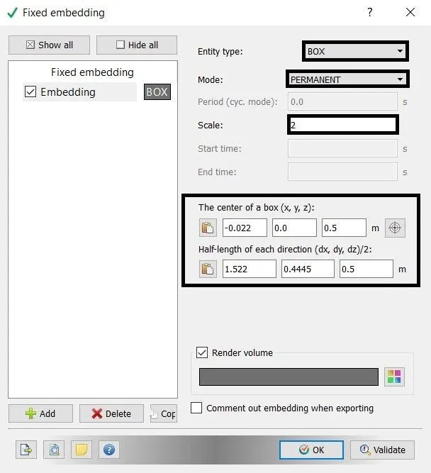
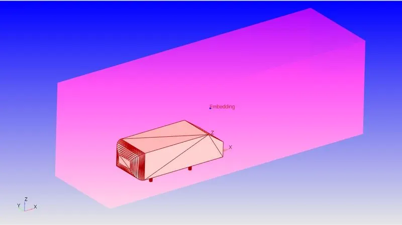
The y-axis and z-axis are calculated by the reference of finer volume resolution area(embedding region).
SIMULATION PROCESS
A. Geometry Preparation:-
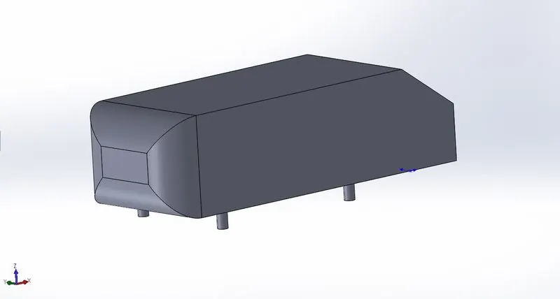
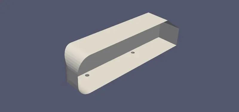
- The Ahmed body is created in SolidWorks based on the given dimension with a slant angle of 35°.
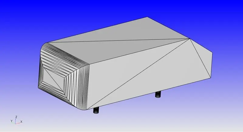
- The model is exported as an STL file and import to the coverage studio.
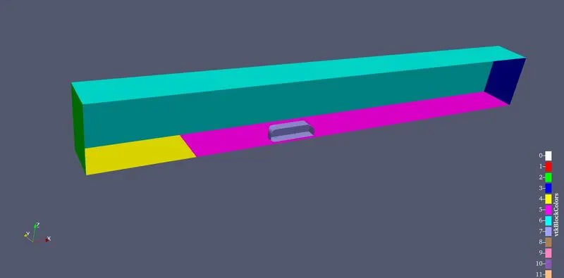
- And then the Virtual wind tunnel is created as per the above-calculated dimensions.
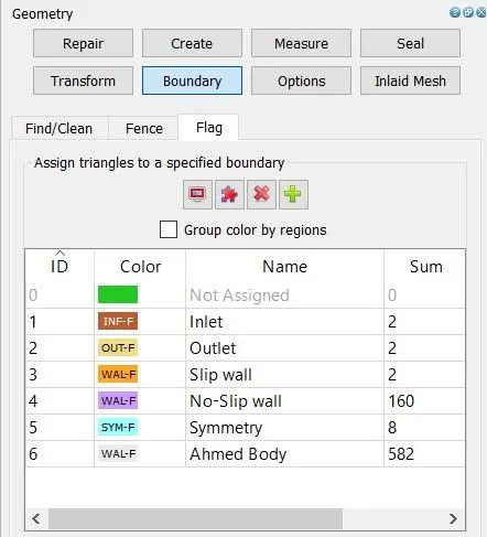
- After creating the wind tunnel the boundary region is flagged.
Boundary Flagging:-
B. Case Setup:-
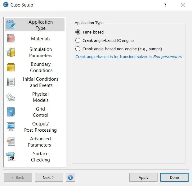
1. Application Type:-
2. Material:-
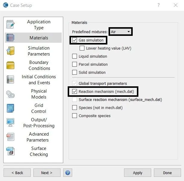
- Gas Simulation - Redlich-Kwong
- Global transport parameters
- Reaction mechanism - O2 & N2
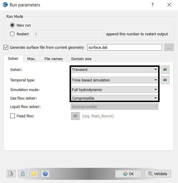
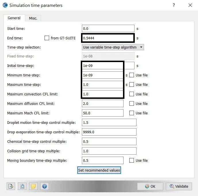
3. Simulation Parameters:-
- Run parameters
- Simulation Time parameters
- Solver parameters
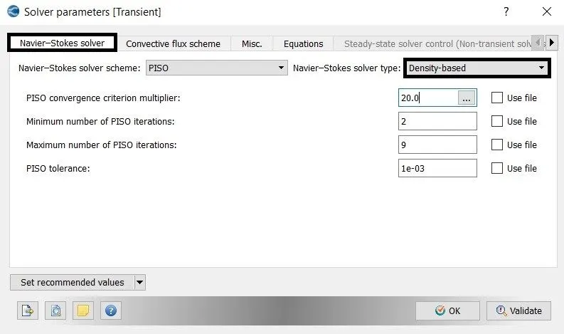
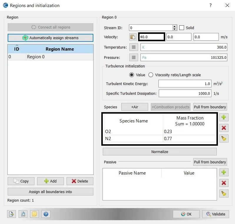
4. Initial conditions and Events:-
5. Boundary conditions:-
- Inlet = Inflow
- Outlet = Outflow
- Slip wall = Slip is used as a velocity boundary condition
- No-slip wall = No-slip is used as a velocity boundary condition
- Top and sidewall = Symmetry
- Ahmed body = No-slip is used as a velocity boundary condition
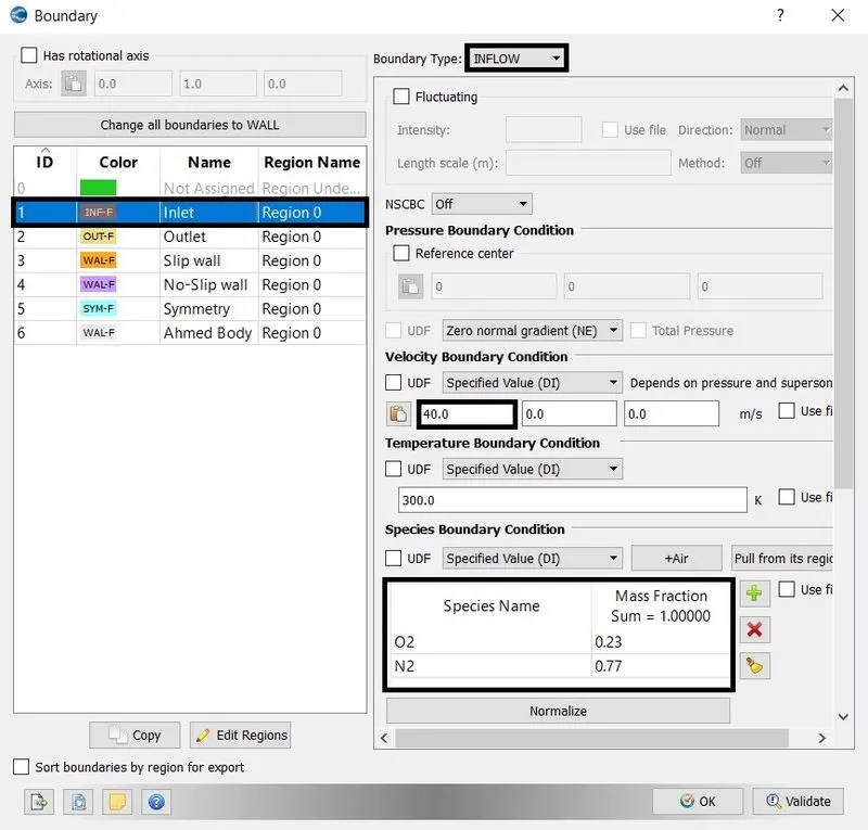
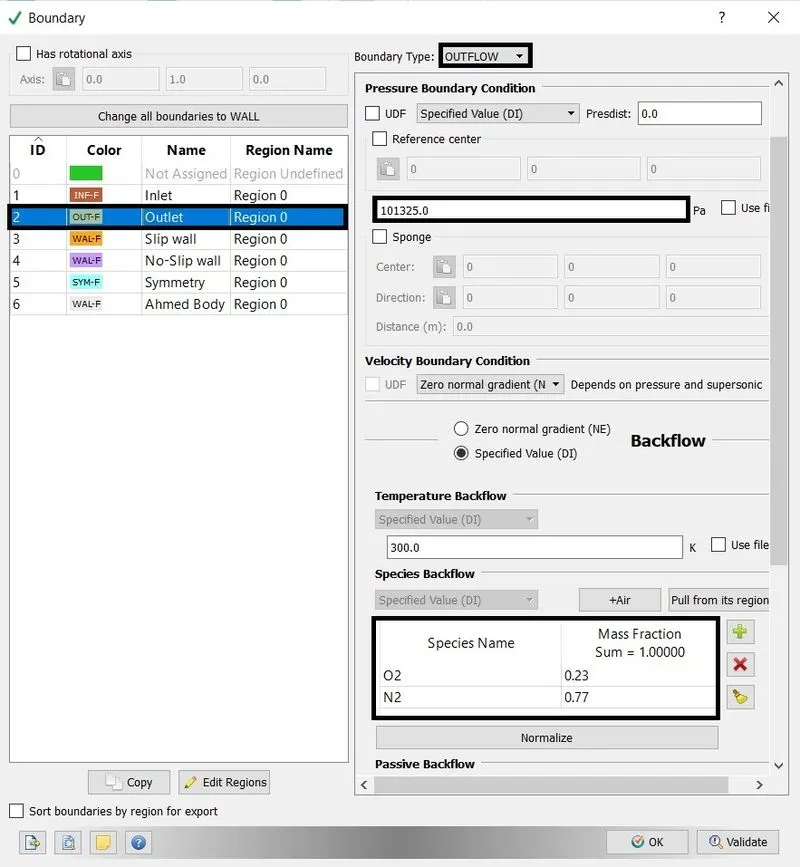
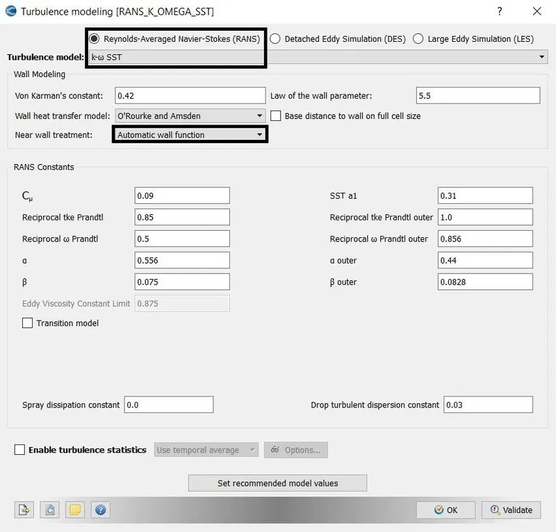
6. Physical models:-
7. Grid Controls:-
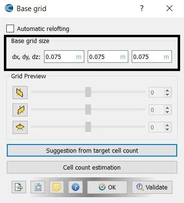
- Base Grid
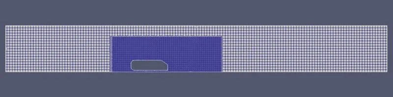
- Fixed Embedding - Box type
8. Output/Post-Processing:-
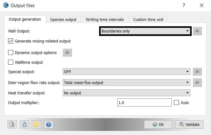
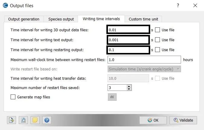
C. Execute the Simulation:-
- The Executable file "mpiexec.exe" and "converge.exe" is pasted in the input files.
- To run the simulation in Cygwin by using the command
mpiexec.exe -n 4 converge.exe restricted </dev/null> logfile &
- After the simulation is complete, the output files can be converted into Paraview VTK in-line binary format to post-process the result in Paraview.
mpiexec.exe -n 4 post_convert_30_msmpi.exe
D. Post-Processing the Result:-
1. Mesh:-
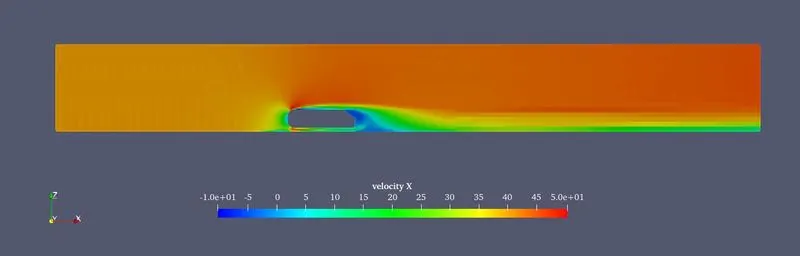
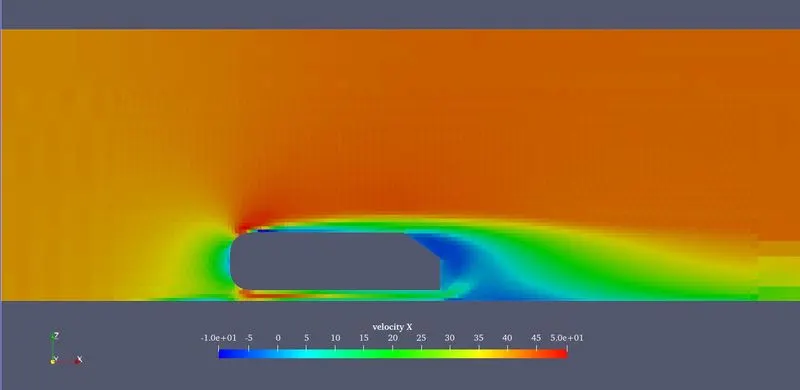
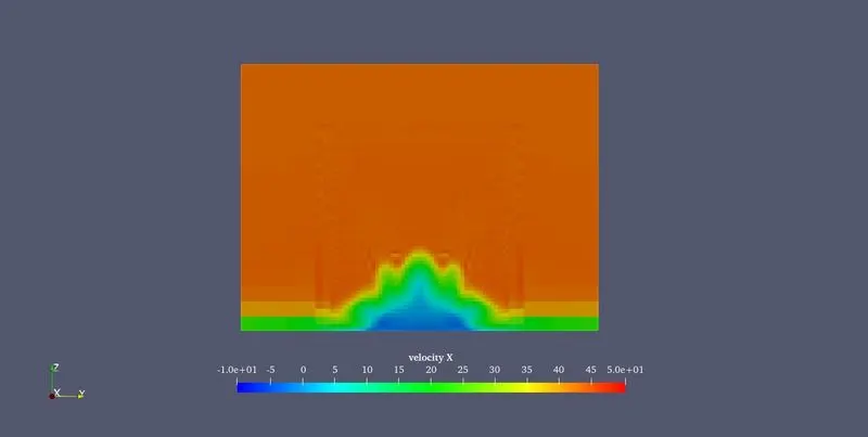
2. Velocity Contour:-
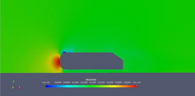
3. Pressure Contour:-
4. Wake Region:-
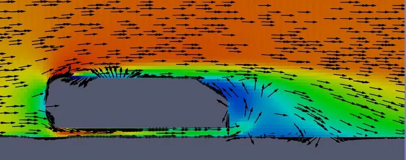
The flow behind the Ahmed body has low velocity and it is recirculated.
5. Animations:-
6. Comparison of velocity plots at different line probes:-
Drag Force calculation and frontal Area Calculation:-
- Calculating drag force in Paraview
- Calculating drag force using wall averaged output.
Formula:-
- `color(red)("Drag Coefficient" = (F_D)/ ((rho*A*v^2)/(2)))`
- `color(red)("Lift Coefficient" = (F_L)/((rho*A*v^2)/(2)))`
where,
`F_D = "Drag force 'N'"`
`F_L = "Lift Force N"`
`rho = 1.1761 kg//m^3`
`"Frontal Area (A)" = 0.0236 m^2`
`"Velocity (v)" = 40 m//s`
In the above formula, the denominator is same so,
`(rho*A*v^2)/(2) => (1.1761 xx 0.0236 xx (40)^2)/(2)`
`color(blue)((rho*A*v^2)/(2) = 22.2047 N)`
1. Paraview:-
Drag and lift force:-
- In Paraview the half of Ahmed body is extracted using the "Extract Body" command.
- And Using the "Extract Surface" command the Ahmed body surface is selected.
- To Generate surface normals and click compute cell normal and apply to calculate the drag force.
- Open the virtual calculator using the filter or icon.
- Change the attribute to "Cell data" and Result Array name as "Drag Force".
- In the scalar dropdown menu, the pressure*Normal_x is used to calculate the drag force.
- The Pressure*Normal_z is used to calculate the lift force.
- After selecting the values they should be integrated over the entire body using the "Integrate Variables".
Frontal Area:-
- The Front area of the Ahmed body is selected using the "Select cells on" feature and extract the surface.
- Select the "Delaunay 2D" and set alpha value 0.05 and apply.
- Integrate the variable and get the frontal area.
Drag Force = 25.1412 N
Lift Force = -118.303 N
`"Drag Coefficient" = (25.1412)/(22.2047) => color(blue)(1.13)`
`"Lift Coefficient" = (-118.303)/(22.2047) => color(blue)(-5.327)`
2. Wall-averaged output data using converge:-
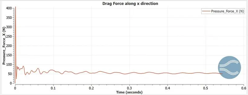
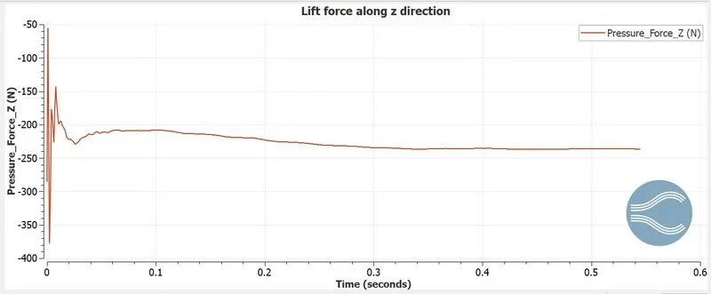
From the output data, the pressure force along the x and z-axis is
- Pressure Force_X = Drag force
- Pressure force_Z = Lift force
Drag Force = 57.51 N
Lift Force = -226.54 N
`"Drag Coefficient" = (57.51)/(22.2047) => color(blue)(2.59)`
`"Lift coefficient" = (-226.54)/(22.2047) =>color(blue) (-10.20)`
Line Plot of Drag Force:-
Line plot of Lift Force:-
Cell Count:-
E. Conclusion:-
| Software | Drag Force | Drag coefficient | Lift Force | Lift Coefficient |
| ParaView | 25.1412 | 1.13 | -118.303 | -5.327 |
| Converge Studio (wall-average output) | 57.51 | 2.59 | -226.54 | -10.20 |
- From that simulation, it can be concluded that the Ahmed body is modelled and simulated.
- The 35° slant angle of Ahmed body is compared with experimental data and simulation data.
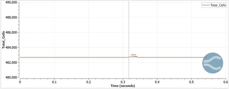
- There is more difference in the experimental data and simulation data because the cell count is 0.48 million cells and the licence is restricted to 0.5 million cells. For accurate results, more computation time and power are required.
- The drag force and lift force is calculated in both ParaView and converge studio.
- In the tabulation, the drag and lift force of converge studio is 2X the paraview. The reason is, in paraview the drag and lift force is calculated as half of the Ahmed body. But in converge studio, the wall output is calculated whole the Ahmed body.
- The Lift force has a negative value and it indicates the lift force acting downward on the Ahmed body.
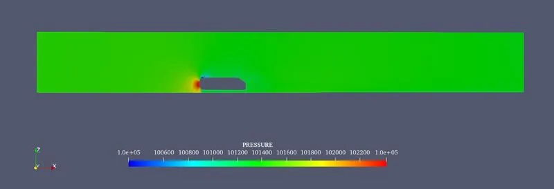
- The Pressure is high in the front region of Ahmed body.
- The velocity is low on the backside of Ahmed body and due to the slant angle the flow of air is recirculated behind the Ahmed body and it is also called as wake region.
Links:-
1. Comparision of experimental and simulation data
2.- Drag and lift force using ParaView
3. Drag and lift force using converge
4. Frontal area