Week - 10 Hyperelastic Material Models

Aim: To perform the material modelling from the data given and calculate the money-Rivlin and Ogden material constants and compare them both using stress-strain data from a Dog-bone specimen tensile test with 100% strain.

Theory:

Hyper elastic material model

Hyper Elasticity: It is well known that there are several types of materials, different from each other in terms of their mechanical behavior.

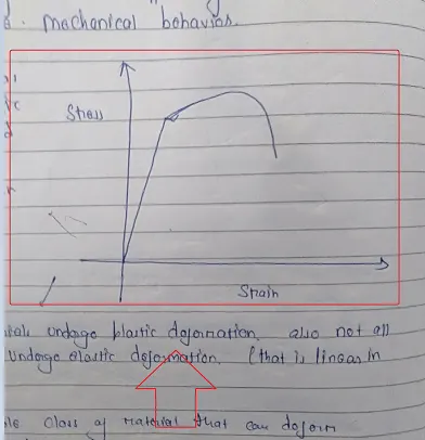
Not all material undergoes plastic deformation, also not all material undergoes elastic deformation that is linear in nature. In fact there is whole class of material that can deform even a strain of 50% or more than that with zero to very little plastic deformation before failure and stress strain response for such material is usually highly non-linear.

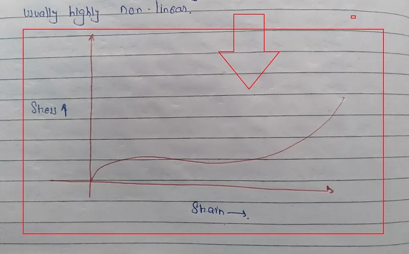
We see every day hyperelastic material in our domestic use and in engineering purpose.

In simple term hyperelastic materials can be defined as type of materials that can undergo Non-linear elastic deformation, typical example of materials that showcase that behavior are rubbers, elastomers, soft tissues, foams and many more. Typically, most soft material behaves in this way and may be classified as hyperelastic materials.

But they still share some similarities with the linear elastic materials regarding the nature of deformation, in both cases the work done on them is stored as internal energy and it is fully recoverable if the deformation is elastic.

Now the question arises why do we need a separate class of material to mimic the behavior of hyperelastic material

The key difference between two is seen in stress strain response from these materials, this response is usually highly non-linear.

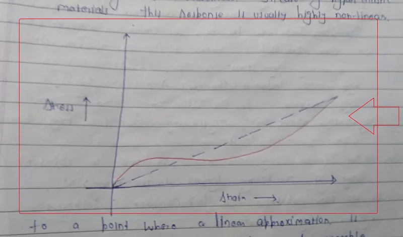
To a point where a linear approximation is inaccurate, take this response for example over here we can see the response is highly nonlinear, with the material having stiff response to begin with that slowly reduces before stiffening again.

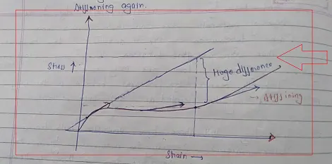
So the stiffness is changing though out the deformation and if one were to mimic the behavior with a linear elastic material, how would they pick the value of elastic modulus considering that it keep changing with strain.

Suppose we use the initial stiffness, which is nothing but the slope of tangent drawn to the initial portion of the curve, in this case let compare the stress response for both the curve at a given strain, here we can see that linear elastic assumption result in very large stress as compared to actual hyperelastic respons, this will result in highly stiff response for the structure and can negatively affect the engineer decision may based on this result.

This is the reason why we need to have a different way of modelling hyperelastic materials, so that we can capture the full complex response of the soft material.

Key characteristics of Hyperelastic material

1. The first thing we notice in this class of material is that they are generally soft in nature as compared to metals
2. Stress-Strain response is non-linear (the slope of the curve which is the instantaneous stiffness of the material) changes with strain.
3. These materials are known to undergo large deformation with very little to no plastic deformation before they fail, this means that the stiffness or stress-strain curve is monotonically increasing until its failure.

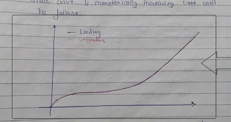
Since they mostly undergo elastic deformation they follow the same path during path loading and unloading this also mans energy is conserved, the work-done in deforming it is all stored as internal energy and is fully recoverable upon unloading.

Most of hyper-elastic material such as rubber, soft tissues are nearly or full incompressible, but other sets of materials such as foams and sponges which are known to be compressible can also be modelled as hyperelastic materials, using special class of hyperelastic models.

As hyperelastic materials can undergo large deformation with very little or no permanent deformation also all the work done in deforming them Is stored as internal energy and is fully recovered upon unloading

This makes the deformation of hyperelastic materials a thermodynamic reversible process, so there behavior follow second law of thermodynamics.

Now let shift our focus toward, how to represent this behavior in form of mathematical equation

As we noted earlier the total work-done in deforming the material is stored as internal energy and all of it is recovered upon unloading

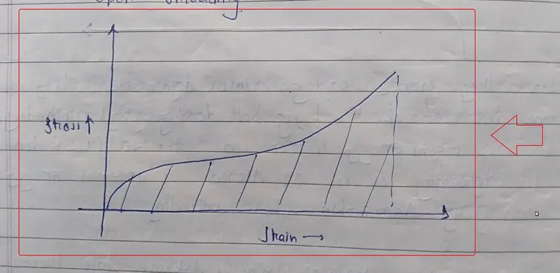
So the area under stress strain curve which is nothing but the strain energy stored in the material, when it is subjected to certain strain. Due to this reason the strain energy function is a perfect choice to be a hyperelastic material model

This energy function is usually defined as the function of strain tensor in the material

Ψ = f(Ɛ)

and the stress developed in the material / body at any given strain is calculated from this strain energy function.

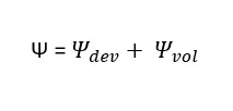
The strain energy function often expressed as additive split of deviatoric and volumetric strain energy.

It is important to note that the stress developed in the body depends upon the type of strain that is present in it.

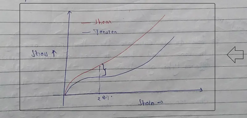
For instance the stress developed in the part at a tensile strain of 20% is different from the stress developed in the same body at shear strain of 20%

So it is important to note mode of deformation that the body is experiencing. In general there are modes of deformation that can characterized the behavior of hyperelastic material namely

Uniaxial tension

Uniaxial compression

Shear deformation

As we see from the chart shown below the value of stress developed in the part at the same amount of strain differ depending upon type of deformation.

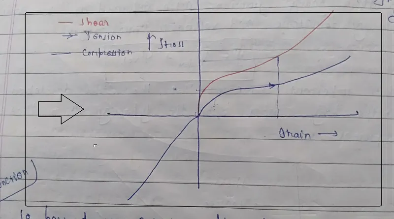
No question comes into our mind that how do we calculate the stress from energy function and how do we differentiate between types of strain.

To understand this we must know what the strain tensor look like for each of these deformation cases, this can be done in two ways

The first method uses principal stretches

Let start with cube of side edges = l is stretched in one direction, when it stretched to size ly the curve will shrink in other two direction to conserve the volume component due to incompressibility.

The ratio of final length of cube to its initial length are called as principal stretches

Principal stretches

λx = lx/Lx

λy = ly/Ly

λz = lz/Lz

physically they tell us to what extent and in what direction did the material change its dimension during deformation.

For instance at different state both the initial and final length of cube are same

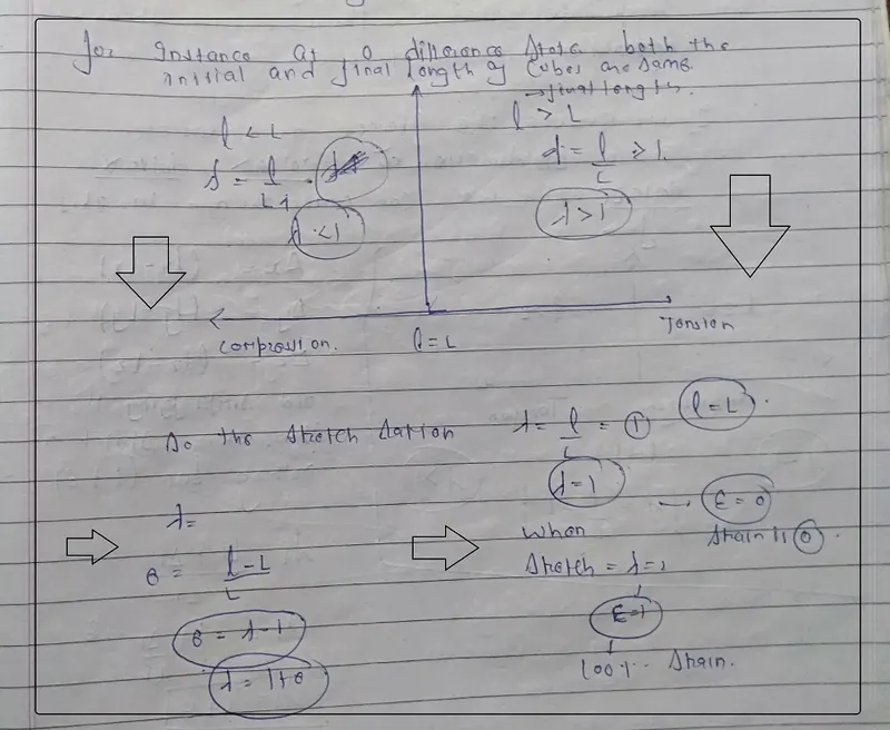
For compression stretch λ < 1 (if part is compressed in one direction its final length is going to be smaller than its initial length and hence the stretch ration is less than one)

For Tension stretch λ > 1 (similarly If part is elongated in one direction its final length is going to increase or more than its initial length)

Since those stretches are defined in principal direction there are no shear deformation in this direction.

If we measure the changes in dimension in 3direction as deltaX, deltaY, deltaZ, then we can write them in this form

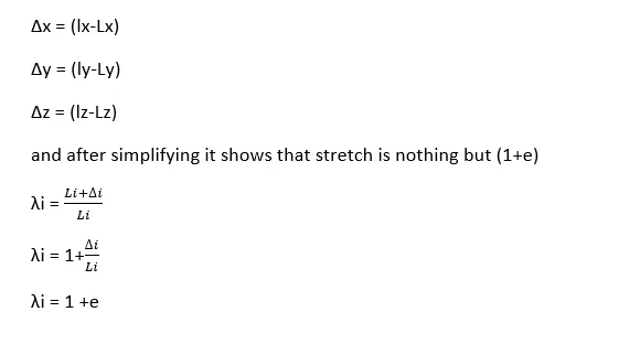
so stretch is λ = 1+e

For λ = 2 engineering strain e = 1 means 100% (length changes to twice)

this way one can relate any type of deformation in the form of principal stretches and use them as a way of representing the strain tensor.

Principal stretches are not the only way of representing the strain tensor for all modes of deformation, another very popular way of doing this is by using the strain invariants.

The strain variants as name suggest, don’t vary as the reference coordinate system changes, so whether the body is undergoing tensile or shear or combined loading its state of strain can be described using strain invariants.

Using one of two methods one can distinguish between different modes of deformation due to this reason they are commonly used in defining hyperelastic material model

Ψ = f (λ1, λ2, λ3)

Ψ = f (l1, l2.l3)

Some of the commonly used model to show how hyperelastic model are formulated

Neo-Hookean model is the simplest form of hyperelastic material model, this function use linear relation between strain energy potential and first strain invariants.

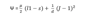
μ is the initial shear modulus

d is the 2/initial bulk modulus

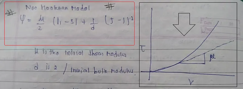
One thing is to note that ALTHOUGH THE EQUATION IS LINEAR, invariant itself is non-linear function of strain, so this is still nonlinear model, it has only two material constant the initial shear modulus μ (so it has unit of stress) and the incompressibility constant, which is nothing but 2/initial bulk modulus

Note that when two different material is modeled with Neo-Hookean model the value of μ and d for both the cases will be different, and this is how we can differentiate between different materials.

Mooney-Rivlin model is commonly used for hyperelastic model

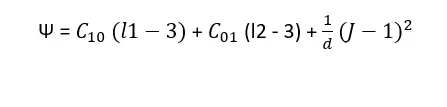
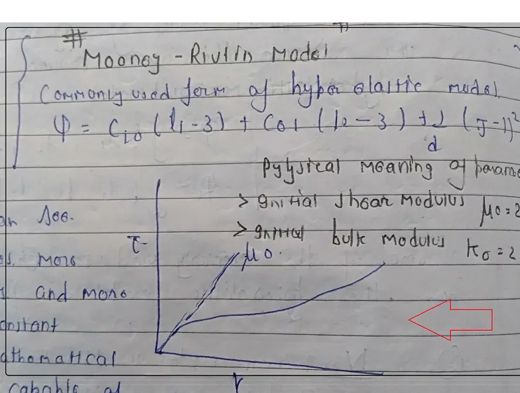
As we can see here this involves more invariants and more material constant, due to its mathematical nature, it is capable of modeling material behavior that is more complex and slightly more non-linear, once again the material constant is related to initial shear modulus of the material and again the incompressibility parameter is related to the initial bulk modulus as 2/d

The Mooney Rivlin model that we see over here is just one form of it, in facts you can add more terms to it, to have 5 terms or even a nine terms Mooney Rivlin model, they come in handy when the material is highly nonlinear and may require more polynomial terms to capture the behavior.

The OGDEN MODEL is another commonly used form and this one is defined using principal stretches

Physical meaning of material constant

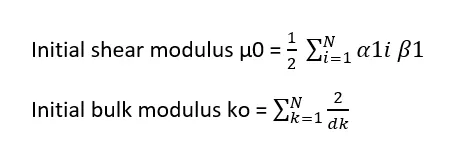
α is dimensionless, nonlinear constant

It can be formulated by one or more term, usually the nonlinearity of the model increases as we use more terms, the deviatoric component of the model has two material constant per term, volumetric term uses one constant per term.

Again incompressibility constant d = 2/initial bulk modulus

Hyper elastic material model that is used specially for modelling compressible foam material

Ogden foam model which is used to model compressible foam materials

Its formulation look very similar to the ogden model, but here you can notice that both the deviatoric and volumetric term are tightly coupled, this make the model suitable for capturing the deformation, but here the volumetric deformation is not negligible as compared to the deviatoric deformation.

This is one of example of tight coupling between the deviatoric and volumetric terms in fact there are several other form that are available to the model such material depending upon how nonlinear they are or even whether they are incompressible such as rubber or compressible such as foam.

Some model such as Odgen or Mooney Rivlin can have multiple term in it, but how we can decide when and how many terms are supposed to used in modelling a material, let looks at what these term will actually do, let take this response as an example

Let take this response as an example

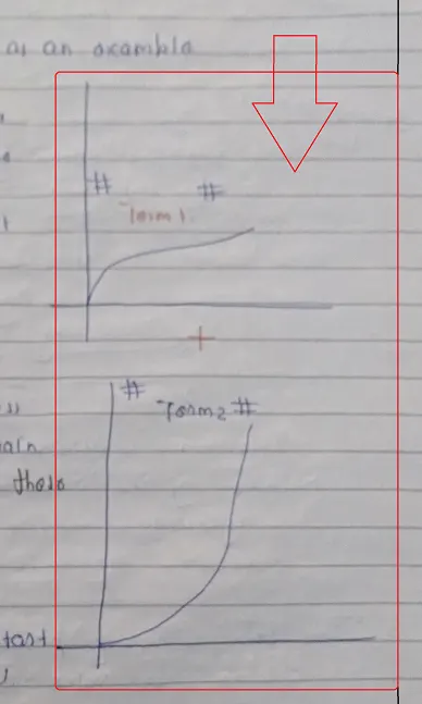
Say the 1^st term has convex upward response, where the material start with stiff response and reduces at higher strain and second term has a concave upward response, where the material stiffness is increase with the strain, so the combination of these two mid-terms will look like this

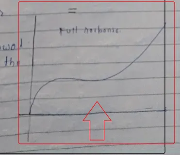
Full Response

As one model is more dominating at start, we can see the material start with a stiffer response the stiffness reduces for a bit followed by an increasing again in the stiffness.

Most of the elastomers have very complex microstructure with multiple polymer chain acting as a load bearing component and each term in the model is represent one such chain structure, so in most cases when you see response like this it indicates that we will need to pick a multiple term model to represent its behavior.

Note: In case of incompressible form a proper usage of incompressibility term is very important

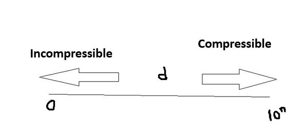
This term is related to the initial bulk modulus of the material and based on this definition as the value of d decreases the material tends to be more incompressible, this term is usually positive and doesn’t have range, but value of 0 indicates that material is fully incompressible.

In some cases, if we need to introduced a small amount of compressibility to make it nearly incompressible, we need to pick a very small value of d.

One recommendation is to set the initial bulk modulus to a fewer order of magnitude about 100 to 1000 times higher than the initial shear modulus and calculate the value of d accordingly.

Calibration of Hyperelastic material model

In general irrespective of material model we perform the simple controlled experiment. To measure a material response to the applied load and then we can calculate the material property from this measured response.

In case of metal we perform simple uniaxial tension test on a dogbone specimen and once we get the data points for stress strain we fit a straight line to this data which gives us slope and the x-intercept

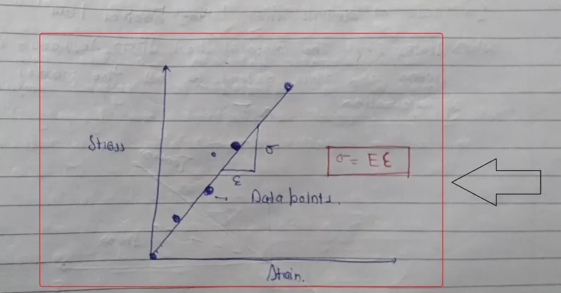
Since materially usually have zero stress deformation the X-intercept is just zero, so we just left with calculating slope which is nothing but Young’s modulus of the material.

In order to calculate the poisons ratio, we need to perform a separate experiment but the idea is still same, we try to fit the approximate equation to the measured data and calculate the material property.

Stress tensor of the material have two types of stress

Normal stress & Shear stress

In case of Normal stress the material can undergoing either tension or compression which are again two different mode of deformation.

So overall there are three modes of deformation seen in the material and one must understand how the material behaves in all 3 modes of deformation.

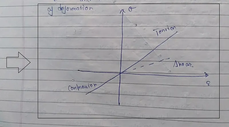
Also metal has same stiffness in tension and compression even the shear response can be calculated from the uniaxial response and the solution is unique too.

So in case off metal one can actually predict the full deviatoric behavior of the material by measuring its response in only one mode of deformation.

However this is not the case for the soft material, soft material such as elastomers, rubbers and soft tissues have nonlinear responses in all the three modes of deformation, due to this the stiffness in all the three mode of deformation is different.

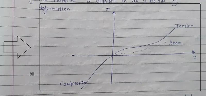
Although in theory on can still calibrate all model parameter using data from one mode of deformation but the solution is not unique, due to non-linear nature, so one can’t accurately predict the full deviatoric behavior of hyperelastic material by measuring response in just one mode of deformation.

So material must be tested to measure the response in all three mode of deformation which are

Uniaxial tension

Uniaxial compression

Simple shear

These 3 modes are required to accurately characterize the deviatoric material behavior of hyperelastic materials. There is fourth mode of deformation which also need to be measure to calibrate the volumetric behavior. In this case material is subjected to confined compression, where the material is constrained in all direction except the loading direction.

This way the stress state created in the material is predominantly volumetric, the change in volume calculated from the applied load and the hydrostatic pressure is measured using load cell to update the hydrostatic pressure generated due to control change in volume.

One important thing is to note in all these cases the material is undergoing homogeneous deformation meaning the stress is uniform in all points of body, this is very important in calibrating the hyperelastic material model, but it is not always practical to achieve such a state during controlled experiments, this can be due to such as improper gripping of the sample in testing, apparatus or difficulties in procuring the sample especially in case of soft tissue and sometimes the material response is even affected by the frictional forces between the sample and the apparatus. The problem with using such data is that there are additional forces registered in the response due to this calibrated material will either be stiffer or softer than the actual response.

Let’s look each modes of deformation and how are they tested

Uniaxial Tension: one of the most popular method, as it easier to conduct, in this test the sample is hold rigidly between two clamps one of the clamp is held fixed while the other is moved to create a state of tension and the reaction force is measured by the load cells, on thing worth to notice is that in this type of testing the sample is usually cut in the form of dog bone and not a simple rectangle, this is because when a rectangular sample is rigidly held between the clamp, the resulting deformation is not homogeneous and can’t be used for calibrating the material model.

So instead of this a dogbone specimen is used in this case, the material is held rigidly at the wider ends but due to the difference in cross-section the material at neck is relatively free to deform, so it creates nearly homogeneous deformation in this region this is still not fully homogeneous, but practically this is good enough.

Compression test: Generally a cylindrical sample is sandwiched between two plates and one of the plate is held at rest while other moves such that it creates a state of compression, but issue with this method is that if there is friction between the plate and the sample, then sample is not free to move at the interface and as a result it start bulging at the centre which creates non-homogeneous state of deformation. So the sample and plate is well lubricated before testing to avoid this behaviour but this will cause trouble in holding the sample in place, so it wouldn’t slip away from the apparatus which is both a waste of experiment and damage of apparatus.

As an alternative in case of fully or nearly incompressible materials, we perform another type of test called as biaxial test this is neither uniaxial nor compression, so how this is considered as substitute

Since the material is stretched in two directions due to its incompressible nature it undergoes compression in 3^rd direction. Recall from definition of Jacobian that is the product of three principal stresses

J = λ1, λ2, λ3

In case of fully or nearly incompressible materials we can set its value to 1 which lead us to this relation

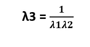
By controlling the value of λ1 and λ2 in our experiment we are able to control amount of compression in 3^rd direction, we can make it simple by using the same amount of stretch in two directions, this way one can mimic the homogeneous compressive response without being affected by this friction.

Note that this relation holds good only for fully compressible materials, in case of compressible material J is not equal to 1 and in fact is function of three principal stretches

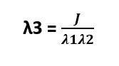
So this relation is no longer user controlled also note that the biaxial tension response is replacement for uniaxial compression test, but the two responses are not equal.

Finally looking at the shear

In case of simple shear it is constant volume deformation where the two sides remain parallel to each other, in general the sample is bonded to two parallel plates and one plate is moved in lateral direction while other one is held constant to generate a state of shear.

The success of this state depends upon the strong bond between the sample and plates to have no slip boundary condition between them such a bond is not easier to have for rubber and tissue, so this method is also not used commonly instead of that we measure another kind of stress state called as pure shear.

The difference between simple and pure shear is that in simple shear, the two sides remain parallel but the sides that are perpendicular to begin with don’t remain that way, so rectangle changes to rhombus.

But in the case of pure shear the sides remain both parallel and perpendicular, so rectangle remains rectangle, but with different dimensions this state is usually achieved in an experiment called as planar tension.

In this case a tall thin sample is clamped along its longest side, one is held at rest and other is moved to create a state of tension.

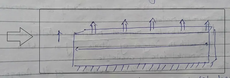
As we notice this is simple to uniaxial tension test. So is it any difference, there is difference in sample, the key here is that the sample is thin and length is almost 10 times the thickness and sample is stretched by doing so deformation along its length due to incompressibility is almost negligible, this creates a biaxial stress state along its cross-section as a result the plane along the diagonal is in a shear state.

Once again this is possible in case of fully or nearly incompressible material and this approximation can’t be extended to compressible material.

This way one can capture the shear mode of deformation in the material without worrying about the failure of bonds at the interface between plates and the sample.

There are typical method used for characterizing the deviatoric behaviour of hyperelastic material.

Note: Just to reinstate that we only need data from at least one mode of deformation to calibrate the material model, however it is recommended to use data from as many modes as possible to accurately characterized the material model, also the calibrated material model is reliable only with in ranges of strain for which experimental data is available, the model can still use outside of the range but the analyst must verify the result and use them with cautions.

Curve fitting for Hyperelastic material

Hyperelastic material are class of material that can undergoes deformation as large as 40% and sustain zero to negligible plastic deformation.

Material such as rubber, elastomers soft tissues foam typically exhibit this behaviour the material in thus class such as common traits such as

Characteristics:

Soft in nature as compare to the metal

Non-linear response

Same loading and unloading curves, this implies that all the work-done in deforming them is conserved and it is stored as internal energy which is fully recovered upon unloading.

The attributes of such material is used in defining their constitutive model in terms of strain energy density, which is the amount of internal energy stored in unit volume of the material.

Ψ = f(Ɛ)

The strain energy density is the function of the strain in the material and the stress developed in it are calculated based on the mode of deformation, so the response can differ depending upon how material is deformed.

So to summarize because of the complex stress-strain relationship of elastomeric materials hyperelasticity is typically define with an equation called a strain energy potential.

Our challenge is to determine these coefficient of the equation in order to characterize our material properties and that’s where experimental data from control experiment come into play.

Typical we perform test in 3 modes of deformation and calibrated or curve fit for hyperelasticity coefficients

These 3 modes of deformation are

1. Uniaxial tension
2. Uniaxial compression or biaxial tension
3. And in shear planar tension

In addition to this we also conduct or performed confined compression test to calculate its volumetric response, together these four data sets comprise a full set of data required to accurately calibrate the hyperelastic material.

In case of material that are either fully or nearly incompressible one may ignore the volumetric data under the assumption that the material is fully incompressible.

It’s worth noting that in practise one may calibrate the hyperelastic model using test data in one of three mode of deformation.

In such cases the model response may be reliable in only that mode of deformation, therefore while it’s possible to calibrate those model using data from only one mode of deformation, but it is highly recommended to used data from multiple or all three mode of deformation.

The calibration of hyperelastic material involve selecting the hyperelastic material model and curve fitting it to the available experimental data.

As a result we are getting constants, which are considered as material properties

There are several hyperelastic material model available, when we perform the curve fitting we are calculating the cumulative mismatch between the experimental data and model prediction and minimize the value for an optimal set of material constant.

The error function is called least square function and depending upon the nature of model, the number of error is

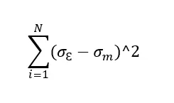
Material constant either a linear or nonlinear regression method is used to minimize it

The minimized value of this error function is called as residue and it can be used to compare the quality of fit between two different model.

Application of Hyperelasticity [1]

Rubbers are generally soft materials that don’t have much resistance to heat and other harsh condition, they are subjected to chemical process known as Vulcanization which makes them stronger and resistant to heat, due to their mechanical properties they are used in wide range of application such as tyres shoes soles toys etc.

Here we calibrate and Validate the material model for one such grade of Vulcanized rubber using a hyperelastic material model.

To do this we will use two sets of data one for calibrating the material model which consist of single deformation mode response and other for validating it against a mixed mode deformation response.

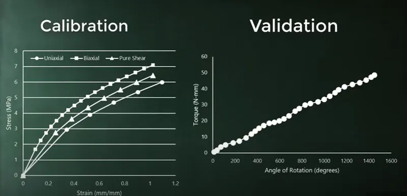
The objective of this example to demonstrate the procedure for calibrating the hyperelatic models and then validating them against a separate test data.

The calibrated test data consist of response measured from three different modes of deformation

The uniaxial tension test, Biaxial tension test, and the pure shear test

Vulcanized rubber is known to be incompressible in nature so the biaxial test data and pure shear test data can be used as alternative for compression and simple shear mode.

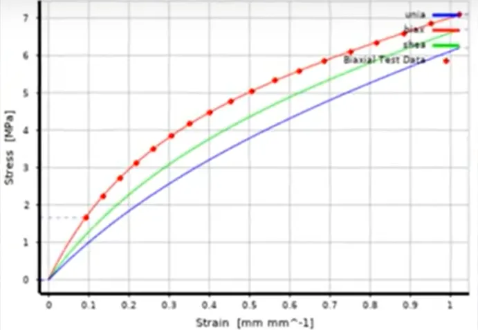
As we seen all three responses are different from each other which is one of the characteristics of hyperelastic materials

As the first step toward the calibration, we pick a model to perform a curve fit

In this example let uses a one term Ogden model we can perform curve fitting using nonlinear regression analysis and calculate the value of μ and α

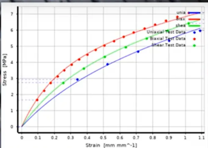
Here is the curve fit result and we can see the quality of fit is pretty good and calculated material constant are μ1 = 4.44 (Mpa) α1 = 1.67 d = 0 (Mpa-1)

Let also calibrate the material by using only one single mode response which is biaxial test data, this is usually not necessary but we will do this to compare both the model responses against the experimental data during validation to see the impact of using full data set vs Just one mode of deformation.

For sake of consistency we will use the one term Ogden model in this case too Here is the curve fit and model parameters

Having only biaxial data (Single mode response)

μ1 = 3.98 (Mpa) α1 = 1.85 d = 0 (Mpa-1)

The geometry of model is rectangular with two holes on both side, the sample is fixed on the one end and it is subjected to displacement of 19mm followed by rotation of 1440 degree on other side

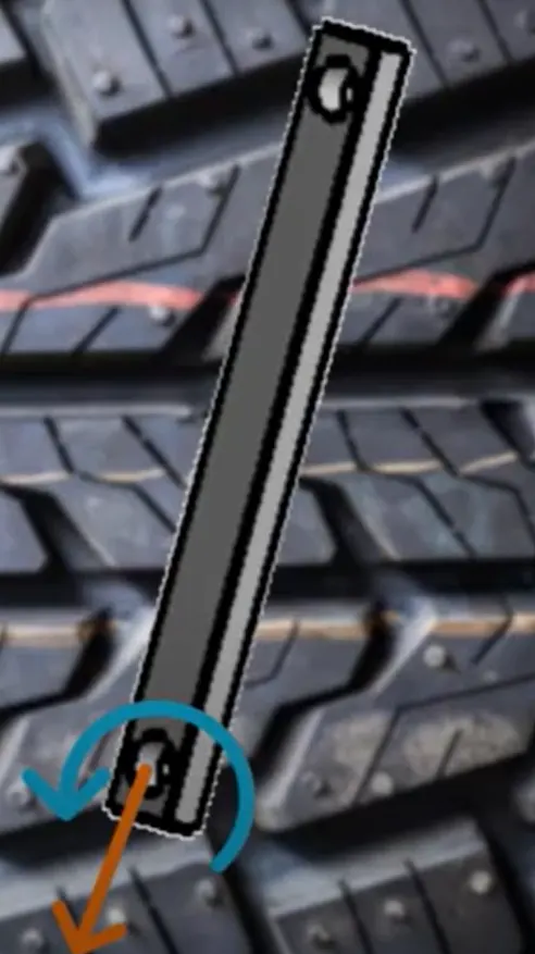
This way a tension torsion state is developed in the sample and the physical material will also tested in the same mixed mode

For validation we will compare the moment reaction forces calculated using both material model against the experimental data.

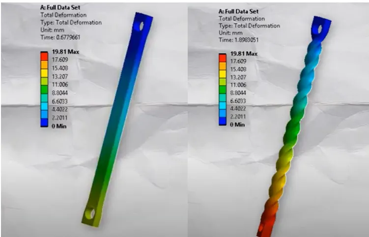
Contour plot for total deformation in sample

The plot is same for both the material mode as this is displacement driven model, as we can see sample undergoes very large deformation under the combined tension and torsion, this is another key characteristic of hyperelastic material, they can undergo large deformation.

Here are the moment reaction calculated by both the models compared against the experimentally measured response.

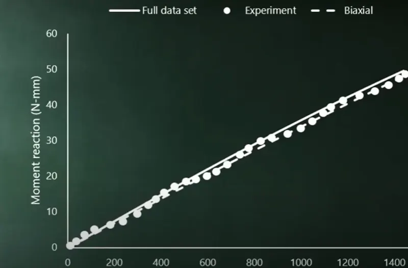
Moment reaction forces (N-mm) vs Angle of rotation (degree)

As we can see they both correlate very well with experimental data, if we carefully observe the response calculated by model using full mode response make slightly better prediction compared to the other model.

This is because full data set includes all the three modes of deformation where as the second mode of doesn’t contain neither the tension nor compression mode, which are two prominent mode of deformation, due to this reason it always recommended to measure the material as many modes as possible to calibrating the material model, also as much as possible it is recommended to plan for some validation test to see how well the material mode is able to capture the mixed mode deformation.

Good example of application of Hyperelasticity

The seals in car door that are popularly called as weather stripping are very useful in sealing the flow of fluids in and out of the car, this include both retailing the air conditioning and heating inside the car also prevent rain water from leaking into the car

The weather stripping is generally made of thermoplastic elastomers which is mix of plastic materials + rubber material, so they are modelled as hyperelastic material.

A key aspect of car door seal design is to see how much sealing pressure is generated when glass window is closed

What is maximum sealing pressure?

In this example we use simulation to asses one such design and how to improve the design if it doesn’t meet the design criteria.

Here is the geometry of window glass seal assembly

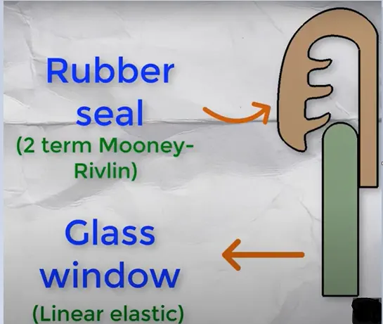
The rubber is modelled using 2 term Mooney Rivlin model and laminated glass is modelled as linear elastic material model, here are the material properties for both the material

Mooney Rivlin Linear Elastic

C10 = 2.59Mpa E = 67Gpa

C01 = 0.65Mpa v = 0.23

D1 = 1.14Gpa-1 G = 27.23 Gpa

Shear modulus = 2(C10 +C01) = 6.48Mpa

Ko = 2/D1 = 1.75Gpa

The initial shear modulus and bulk modulus for the gasket can be calculated from its material constant.

We can see how soft the material is in comparison to the glass material based on their shear modulus, the bulk modulus of rubber (Ko) however is vey large this is because rubber is nearly incompressible, so it will offer a lot of resistance to change in volume in terms of the modal loads and boundary conditions, the seal is fixed along its convex edge and this is where it sits in the window for installation.

We will impose a vertical displacement of 17mm to the glass pane to simulate the window closure

Frictional contact with coefficient of friction of 0.1 is defined between the rubber and the glass parts

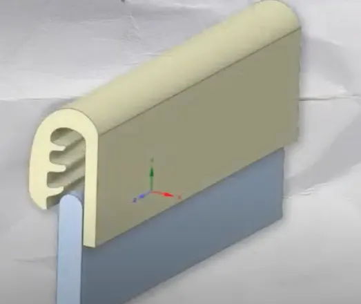
Due to the long planar geometry of the system we will use 2D plain strain model to save computational time

There are no significant inertial effect in play. So we will use static analysis to solve the problem, due to the presence of nonlinear material, nonlinear contact and large deformation this model is nonlinear analysis.

Result from the simulation

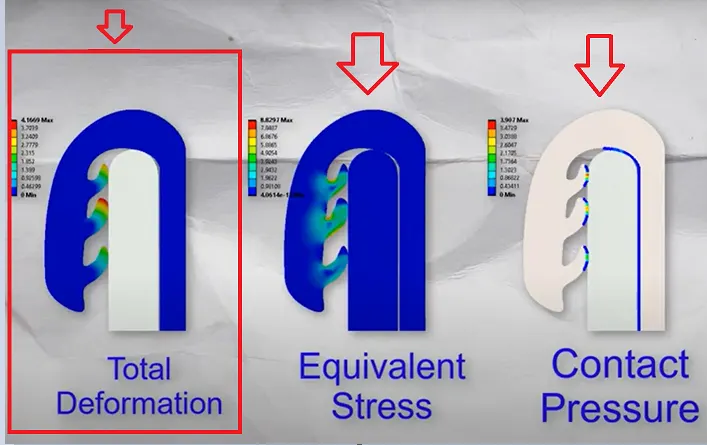
We are looking at the contour plots for total deformation, equivalent stress and the contour pressure generated at the rubber glass interface, we can see that material is undergoing large deformation and we can see where the model is experiencing maximum stress, but most importantly we can see how much contact pressure is generated at the interface, which indicates how much pressure the seal can withstand, in this case it is 3.89Mpa.

But what if we want to improve the design to support more contact pressure

To identify the design changes that may help us, lets look at the contour plot for strain energy to see where it is concentrated.

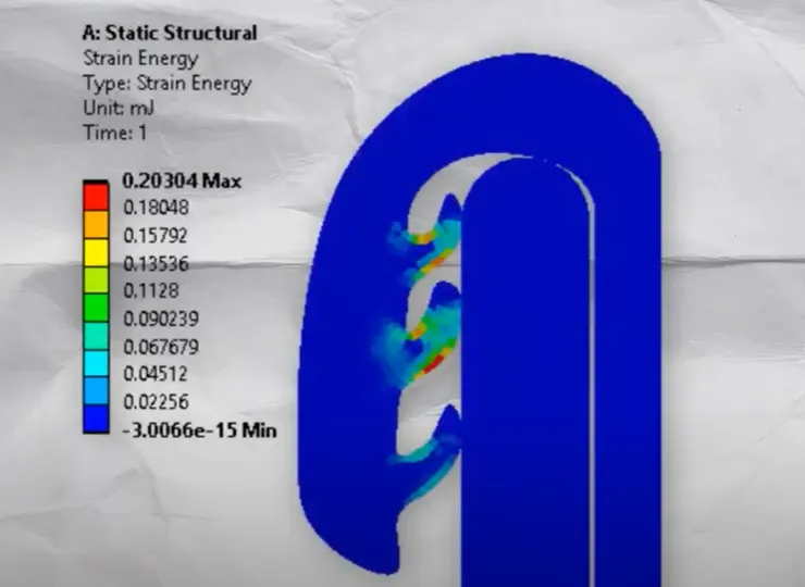
In this plot we can identify the hot spots which are the region that are having most energy concentrated. In other words we should able to distribute the energy in place in a better way, so that they can resist the deformation and offers more contact pressure.

So lets go ahead and make the fins thicker in these region and recalculate the contact pressure for the new design.

Firstly, lets look at the plot of strain energy for a full loading and unloading case

From this plot we can see that strain energy is recovered upon unloading this is another key characteristics of hyperelastic materials

Contact pressure calculated using new design:

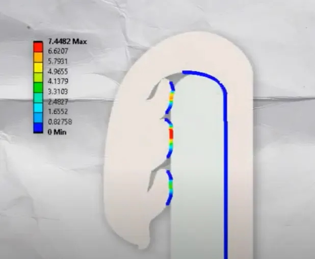
The new design can now withstand of higher pressure of 7.45 Mpa, this is because we have provided a more material in the regions that were having more strain energy density and as a result the material now has more stiffness in those region and therefore offers more resistance to deformation.

This is one of the example to demonstrate the use of hyperelastic material models and how the designers can make use the analysis result in improving the designs.

Procedure:

• Choosing Hyper-elastic constitutive model
• Specifying Experimental data in to the material model.
• Extracting material constant and Fit curve data for each order of polynomial from D3HSP file
• Comparing the fit curve data with Experimental data used in the model
• Extracting stress-strain curve from the simulation (tensile test) for each order of polynomial
• Comparing the stress-strain curve with the experimental data.

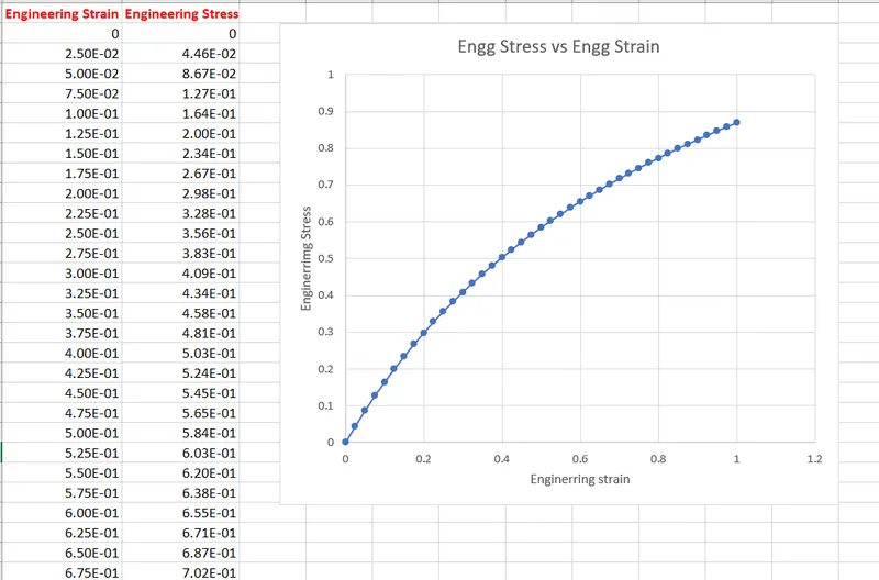
Extracted Experimental data

Deck-Setup

This setup is for tensile test, the material used here is hyper-elastic material. This leads to high amount of deformation, this high deformation leads to Non-linearity in the simulation, here we will carrying out the simulation where inertial effect are almost 0 or negligible, in tensile test specimen is loaded gradually and the deformation happens slowly, so the inertial effects are negligible, so we can go with implicit solving method.

After importing the model, we need to define the material, for that we can use the define curve and we can input the .csv file, which we already prepared with the material curve fitted data, and we will using MAT_077 Hyper-elastic Rubber card. We set the N=1 and we have to define the curve in LCID which is the load curve id, since we are input the engineering stress and engineering strain value we will be setting up the Specimen Gauge length, Width, Thickness as which indicates there is no change in the area of cross-section of the specimen, which basically tells the solver that the defining data is engineering stress and strain and we don’t need to convert it, If we defining the force vs displacement data then we have to specify all the parameters, so that solver can convert the specified data into Engineering Stress-Strain curve. The basic details related to material like density and poisons ratio need to defined, density is taken as 0.001, and poisons ratio of compressible material set to 0.498, for incompressible material the poisons ratio will vary from 0.49 to 0.499, we can’t go for 0.5 value as it leads to numerical instability, so we have to take care about these values before defining them.

Defining Material and Loading curve

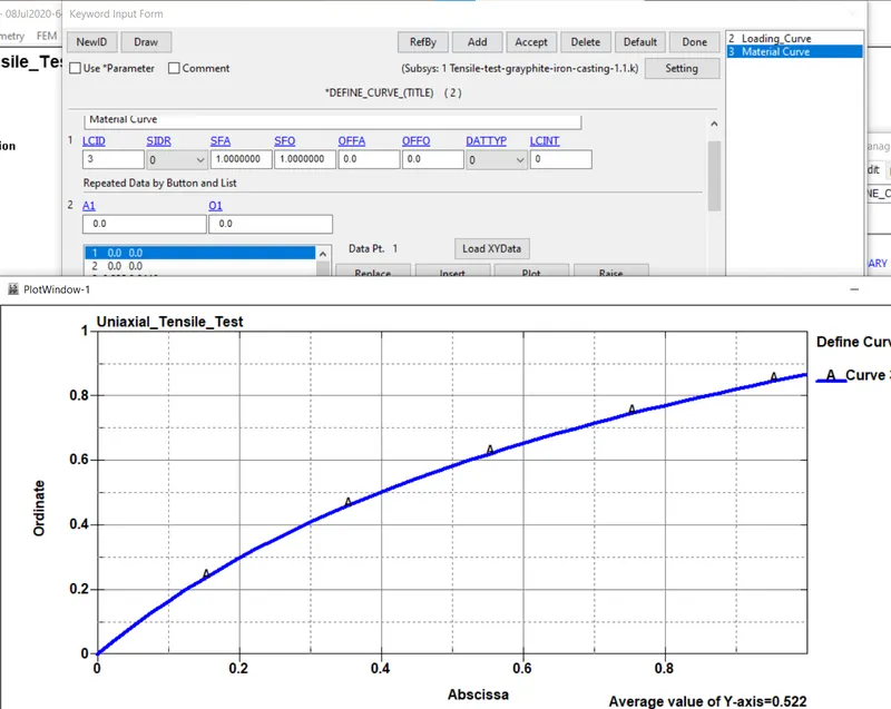
Defining Material curve

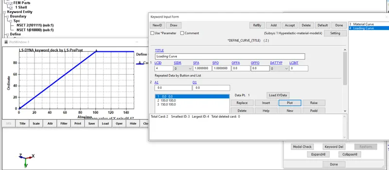
Loading Curve with VAD=2(Displacement based loading)

Setting up Boundary condition and constraints

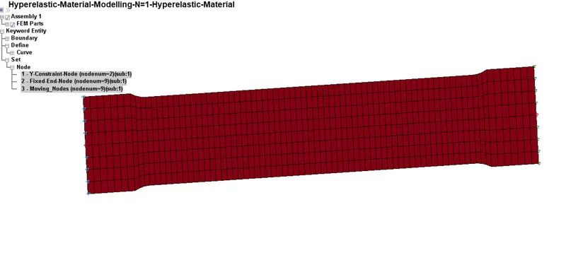
Specimen Constraints and loading conditions

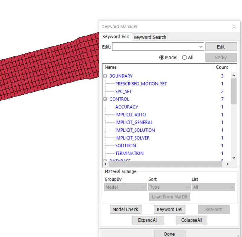
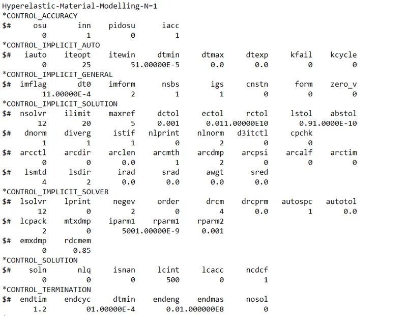
Defining Boundary condition and control cards

Results:

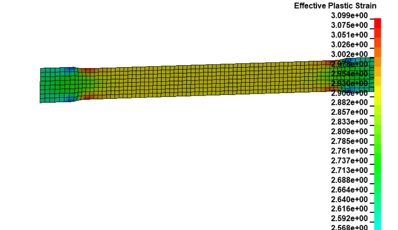
The Mooney-Rivlin constants for each case are stored in d3hsp file

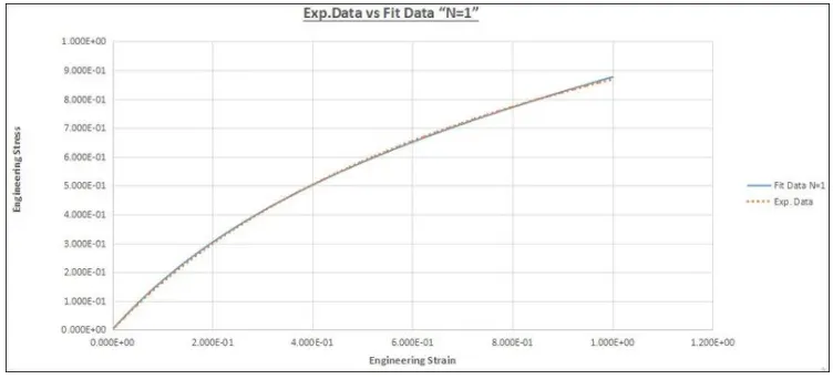
Case1: N=1 First order polynomial

• Mooney constant C01 = 0.1768E+00
• Mooney constant C10 = 0.147E+00

Final fit data from the d3hsp file is generally in Stretch vs True Stress, we have to convert it into Engineering strain and stress

Engineering Strain = Stretch-1

Engineering Stress = True stress / Stretch

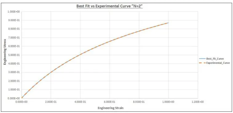
Case 2 N=2 Second order polynomial

• Mooney constant C10 = 0.259E+00
• Mooney constant C01 = 0.4594E-01
• Mooney constant C11 = -0.2092E-01
• Mooney constant C20 = 0.2914E-02
• Mooney constant C02 = 0.1016E-02
• Mooney constant C30 = 0.0000E+00

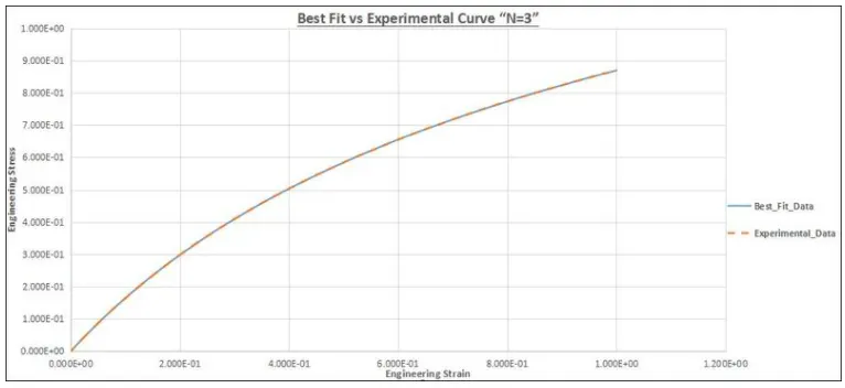
Case 3 N=3 Third Order Polynomial

• Mooney constant C10 = 0.2611E+00
• Mooney constant C01 = 0.4420E-01
• Mooney constant C11 = -0.6074E-02
• Mooney constant C20 = -0.2667E-02
• Mooney constant C02 = -0.9968E-02
• Mooney constant C30 = 0.1565E-03

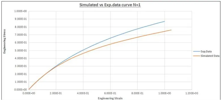
Comparison of Simulation Stress/Strain with Experimental stress-strain data

Case1: N=1 First Order polynomial

Case2: N=2 Second Order Polynomial

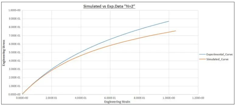
Case3: N=3 Third Order Polynomial

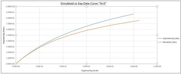
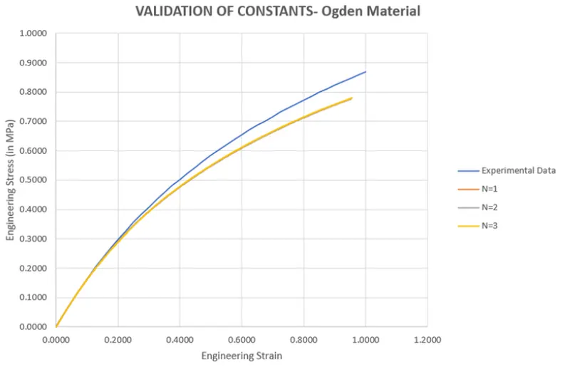
Validation of Constant

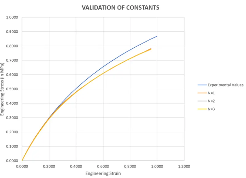
Validation result is different from the Experimental result

For Ogden Material

*MAT_077 or *MAT_OGDEN_RUBBER

Ogden Hyper-elastic model is expressed the strain energy function in terms of principal stretches, where N is the order of the model, usually N takes a number between 1-8 The same procedure is followed for building the Ogden material deck. Since there is 8 orders of polynomial in this material model, here we will use 1,2.3 order of polynomial, for this case Density, Poisons ratio, SGL,SW and ST parameters are set with sane value.

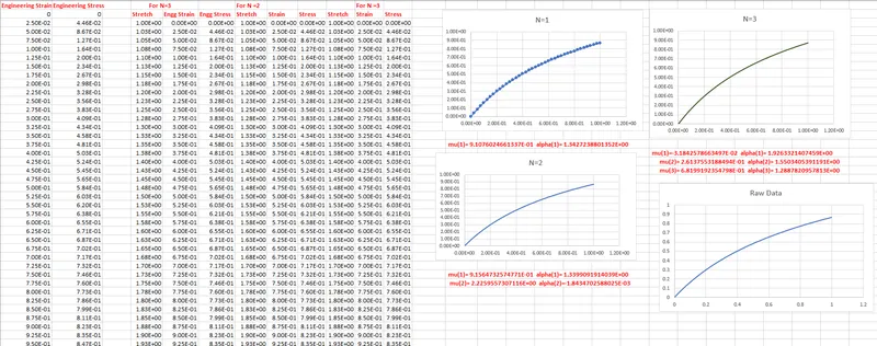
Outcome from Ogden Material

Validation of Constant (mu & alpha)

Conclusion:

• The Mooney-Rivlin and Ogden material constants are obtained from d3hsp file by inputting the value of polynomial N=1 in the material card MAT_77 and MAT_77_O
• The stretch-stress data obtained from d3hsp for both hyper-elastic constitutive model were verified with experimental data and found to be a close fit.
• The simulation result of tensile test for both material models with experimental data showed a slight deviation due to the highly non-linear behaviour of the given hyper-elastic material and the generic value of density and poisons ratio.
• For simulation result both hyper-elastic constitutive models were found to be valid to describe the behaviour of given material data.

Common Mistake during Modelling of Hyperelastic model:

Mistake 1: Calibrating the hyperelastic model using not enough experimental data

There are 2 types of Hyperelastic model

I1 based which includes

Neo-Hookean

Yeoh

Arruda-Boyce

Gent

Marlow/Response Function

Not I1-Based

Mooney-Rivlin

Ogden

Polynomial

Extended tube

Hyperfoam

There is large difference between two, the I1 based model can calibrate using a single loading modes, but the Non I1 based model required multiple test data to calibrate it properly.

So there is huge difference in the amount of work's that needed, lot of us having misunderstanding and and didn't know about this and trying to calibrate Non-I1 based materail model with uniaxial data.

Mistake 2: Not considering Mullins damage

Mistake 3: Using a hyperelastic model when not appropriate

We have to aware that most of material when we considered using hyperelastic are not actually non-linear elastic in the response, they are viscoelastic and if we pick hyperelastic mode then we miss all the viscoelastic behavior that the material would have.

References: Ansys Learning [1]