Week - 10 Hyperelastic Material Models

Objective:

To crearte a hyperelastic material model from the given experimental data and compare the results

Theory:

Hyperelastic material is ideally for elastic material for which stress strain relationship derives from a strain density function. The hyperelastic material is a special case of a Cauchy elastic material. They are characterized by:

1. Can undergo large elastic deformation in the order of 100 to 700% which are fully recovered, i.e., initial shape can be recovered when the load is removed.
2. Are nearly incompressible, i.e., they can change their shape but the overall volume remains constant.
3. A hign non linear stress strain relation is shown.

Many polymers such as elastomers, rubbers and other similar soft flexible materials show hyperelastic behaviour. Hyperelastic materials are mostly used in applications where high flexibility in the long run is required under the presence of high loads Eg: elastometric pads in bridges, rails pads, car door seals, tyres etc.,

Hyperelastic materials are described through a strain-energy density function. The strain-energy density can be used to derive a nonlinear constitutive model (i.e., Stress as a function of large strain deformation ) which are derived by researches are some acceptable models we are using popularly are

• Neo-Hookean (First oder reduced polynomial)
• Mooney-Rivlin (First order complete polynomial)
• Ogden (Second order reduced polynomial).

A Neo-Hookean is a hyperelastic model, similar to Hooke's law, that can be used for predicting the nonlinear stress-strain behavior of materials undergoing large deformations.

A Mooney–Rivlin solid is a hyperelastic model where the strain density function is a linear combination of two invariants of the left caiuch deformation tensor.

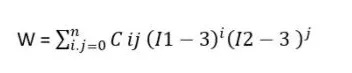
by varying the index values of i and j we can change the constitutive equations and use them appropriately as required.similarly we will be having multiple co efficients of C, This changing of index is basically changing the order of polynomial of energy density equations.we need to find out the coefficient of these material model for a different order of a polynomial and extract the best fit curve data to compare it with the materail curve.

Procedure:

Case setup & Exectution:

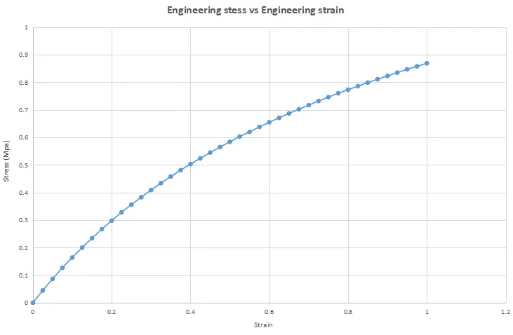
1. The given image consists of Engineering strain and stress values which needed to be imported in to an Excel sheet.

2. Engineering stress vs strain values are plotted upto strain rate of 100% which is 1.

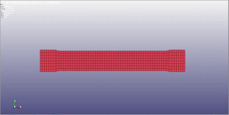
3. Importing the given tensile_test_mesh.k keyword file into LS-PP

4. Assigining Material and Section to part:

• For assigining the material the following steps are followed Keyword manager `rarr`All `rarr`Mat `rarr` Select the material card, here different material properties like mass density, youngs modulus, poisson's ratio and other recommended values are given
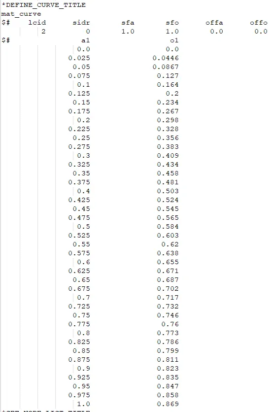
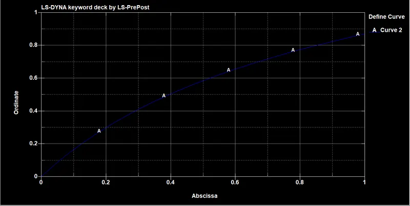
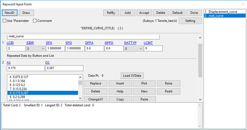
• The values from the given Engineering strain and stress are taken, inputed into the model through define curve
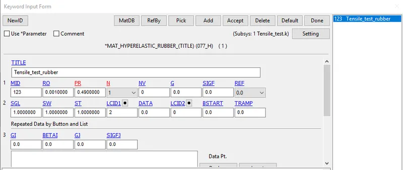
• MAT_77_Hyperelastic_rubber is selected. with density of 0.001 `g/(mm3)` and poisson's ratio of 0.49 is given.

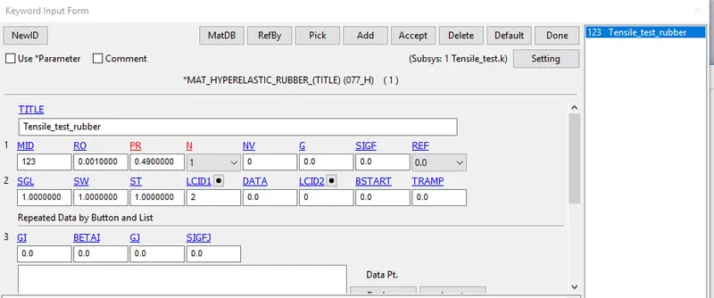
• The parameter N in the Mat_77 cards refers to the order of polynomial for which the constants are required to solve.This involves N1.N2 and N3 cases where the constants are solved along with strtch and true stress data.
• N1 solves for Two polynomials C10,C01
• N2 solves for six polynomials C10,C01,C11,C20,C02,C30
• N3 solves for six polynomials C10,C01,C11,C20,C02,C30

The SW, SGL and ST parameters are set to unity since we have a stress-strain load curve where as in the case of force-displacement data requires specimen dimensions.

Section creation:

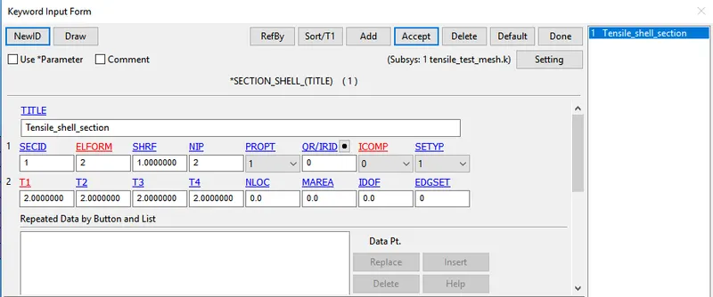
• Shell section is needed to be defined by selecting Keyword manager `rarr`All `rarr`Section `rarr`Shell
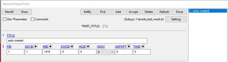
• Here the solid selection with element formulation 2 is defined with the thickness is given as 2 mm

• For creating the part Keyword manager `rarr`model `rarr` part is used , then the respective section and material is assigned to it.

5. Boundary conditions:

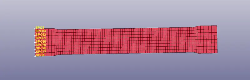
For testing a model for tensile test, we need to fix one end and give diplacement to other end.

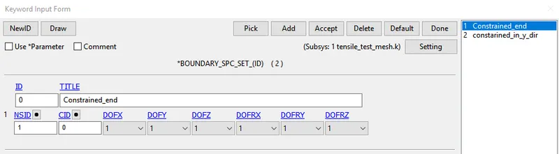
Creating SPC:

A Set of Spc is created at one end constraining all Dof's

Defining Prescribed motion set:

Node set is created at the opposite end in which the Spc is created by Create entity `rarr`Set nodes

In define curve keyword, we need to specify the displacement nodes by Define `rarr`Curve

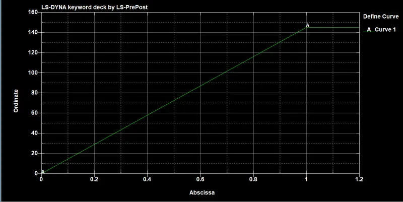
Since the stretch ratio is taken as 100% here

`epsilon = lambda - 1`

`implies epsi = 2-1`

`implies epsi = `(dell)/L = 1` , here L = 145

Displacement ordinate is scaled as 145

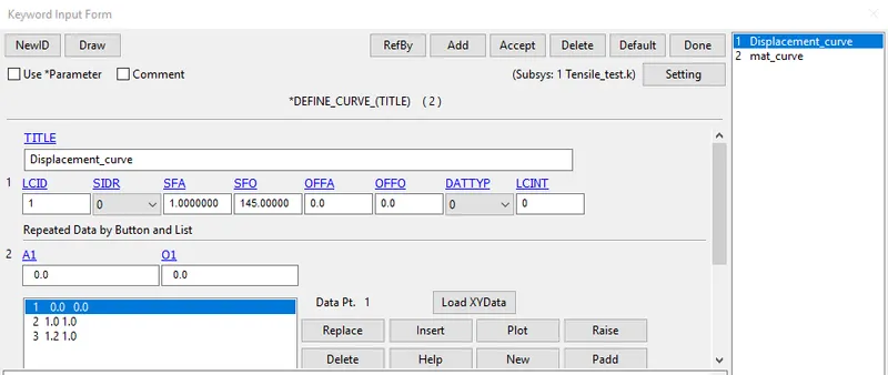
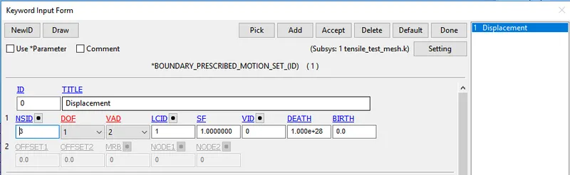
Here VAD is selected as two which refers to displacement.

6.Control Cards:

In LS prepost generally the solver used is Explicit, to perform in Implicit solver the following keywords are needed to be defined to switch from implicit to explicit

i.Keyword manager `rarr`All`rarr` control `rarr` Implicit_Auto

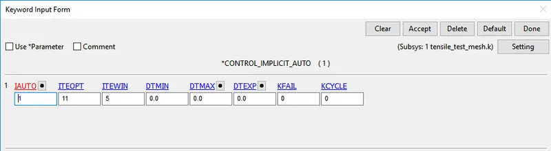
CONTROL_IMPLICIT_AUTO card is used for automatic time step control during implicit analysis. Input value for Automatic time step control flag = IAUTO = 1.

ii.Keyword manager `rarr`All`rarr` control `rarr` Implicit_General

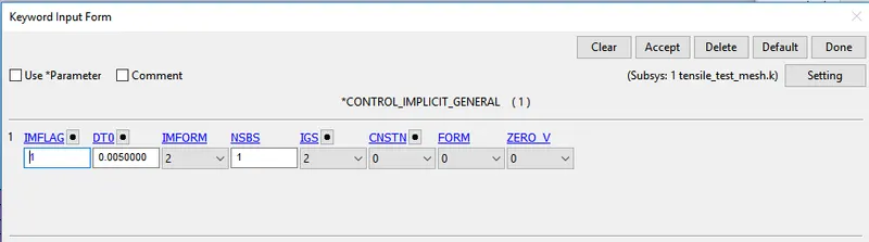
• CONTROL_IMPLICIT_GENERAL card is used to activate implicit analysis and define associated control parameters. This keyword is required for all implicit analyses.
• The input value for IMFLAG=Implicit/Explicit switching flag = 1 (implicit analysis)
• DT0=Initial time step size for implicit analysis = 0.005.

iii.Keyword manager `rarr`All`rarr` control `rarr` Implicit_Solution

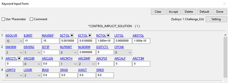
CONTROL_IMPLICIT_SOLUTION card is used to specify whether a linear or nonlinear solution is desired. The default values are set as it is in the card.

iv.Keyword manager `rarr`All`rarr` control `rarr` Implicit_Solver

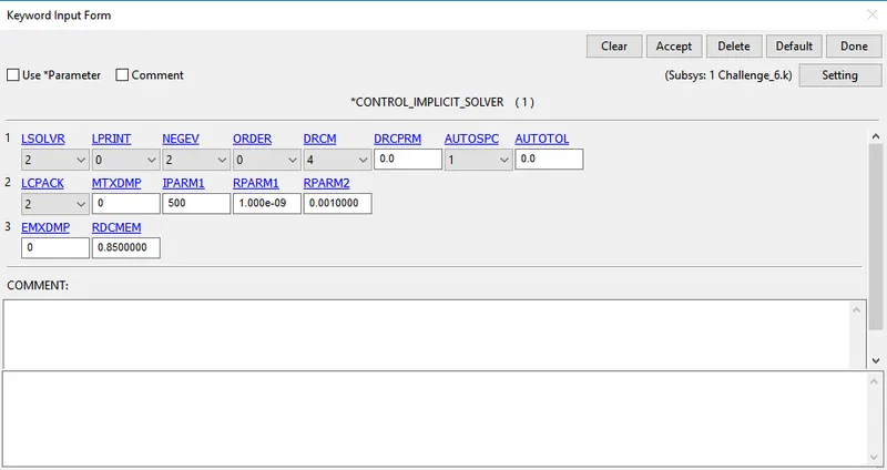
CONTROL_IMPLICIT_SOLVER card is used for implicit calculation.

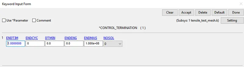
v.Keyword manager `rarr`All`rarr` control `rarr` Termination

7. Output Request:

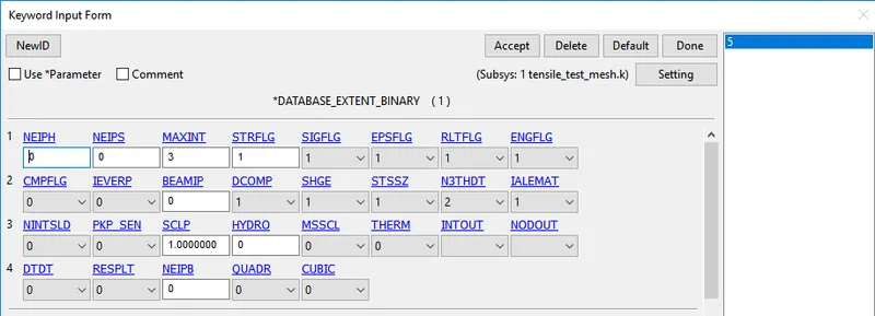
• Keyword Manager `rarr`Database `rarr` Extent_binary with STRFLG = 1 is given , this will compute the elastic strain in the model

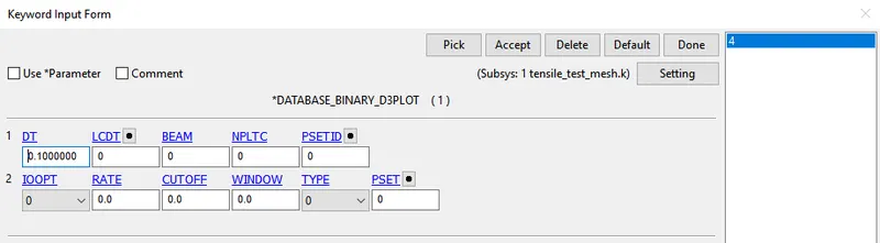
• Keyword Manager `rarr`Database `rarr` Binary D3plot `rarr` DT 0.1, this command prints the output at the end of each 0.01 ms

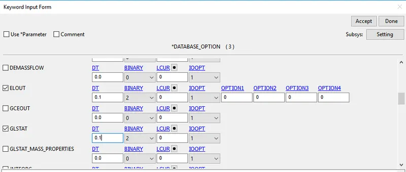
• Keyword manager `rarr`All`rarr` Database`rarr` ASCII_option from which GLSTAT,MATSUM and ELOUT option is selected with DT= 0.1 ms
• GLSTAT is defined with DT=0.01 ms which gives the output of energies such as Internal energies, kinetic energy & other types of energies

Run the simulation

• The keyword is saved in a separate folder and it is opened in Ls-Dyna manager

Results:

Case 1: N=1

With the above mentioned procedure the model is made to run with N=1 in the material card

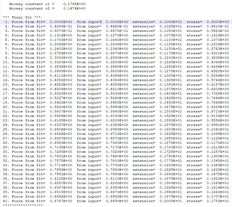
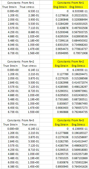
From the d3hsp file, Mooney-Rivlin constants are obtained along with the stretch and true stress values

Mooney constant c1 = 0.1768E+00

Mooney constant c2 = 0.1474E+00

from the stretch and true stress values engineering strain and stress can be calculated by

Engineering strain = Stretch (`lambda`) - 1

Engineering stress = True stress / 1+Engineering strain

Case 2: N=2

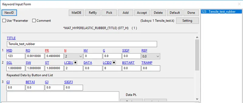
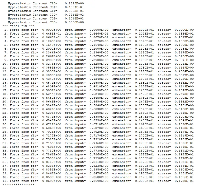
From the d3hsp file, Mooney-Rivlin constants are obtained along with the stretch and true stress values

C10 = 0.2595E+00

C01 = 0.4594E-01

C11 = -0.2092E-01

C20 = 0.2914E-02

C02 = 0.1016E-02

C30 = 0.0000E+00

Similar to the above mentioned case engineering stress and strain needed to be calculated

Case 3: N=3

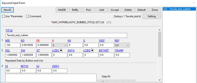
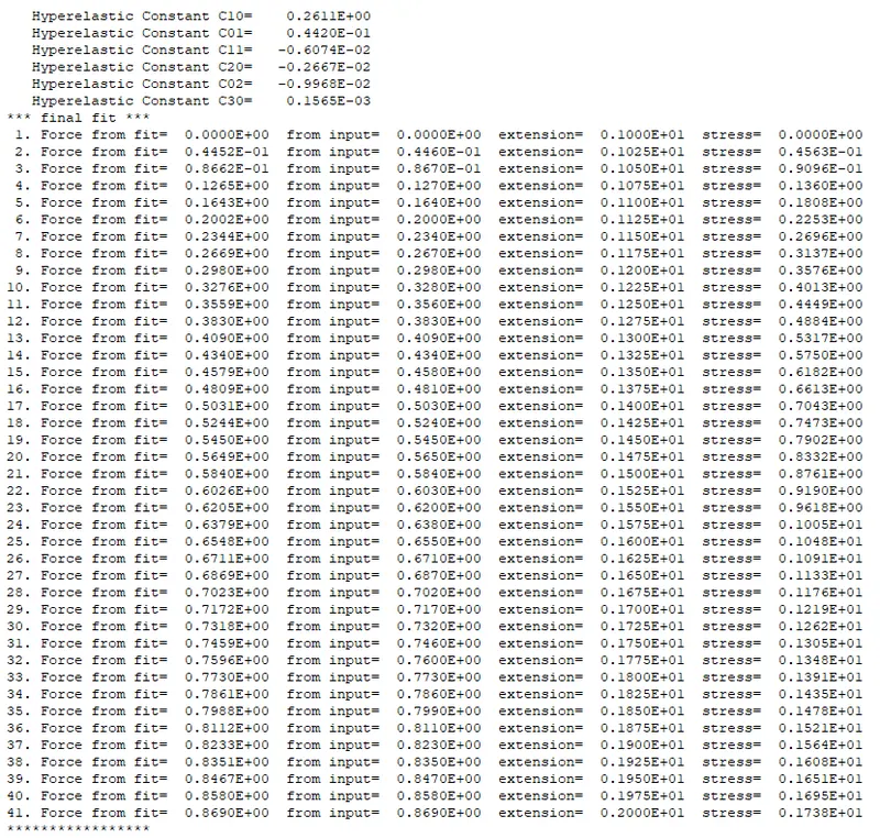
From the d3hsp file, Mooney-Rivlin constants are obtained along with the stretch and true stress values

C10 = 0.2611E+00

C01 = 0.4420E-01

C11 = -0.6074E-02

C20 = -0.2667E-02

C02 = -0.9968E-02

C30 = 0.1565E-03

Similar to the above mentioned case engineering stress and strain needed to be calculated.

Converted Values:

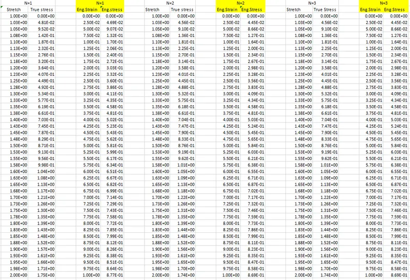
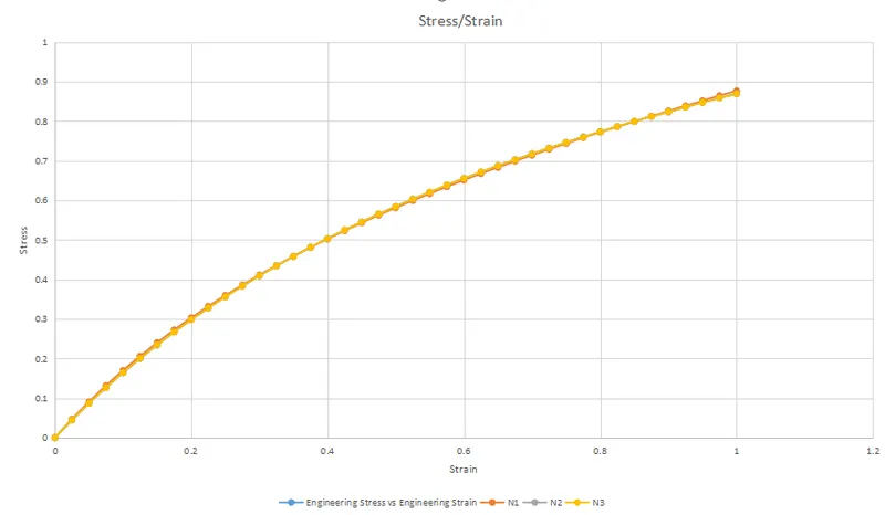
We can see from the graph that the constant values obtained from the d3hsp file is fitting with the original data from this we can conclude that all the constants will give similar results compared to the original data.

Material validation:

To validate we need to key in the constants (C1 and C2 , C10,C01,C11,C20,C02,C03) which are obatined from simulating the material with N1,N2 and N3

• Validation for Case 1: In the *MAT_HYPERELASTIC_RUBBER_ by keeping N=0 we can input the mooney-rivlin constants obatined during case 1

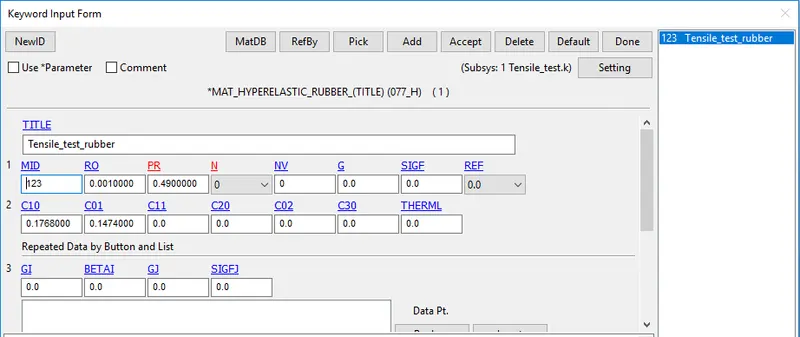
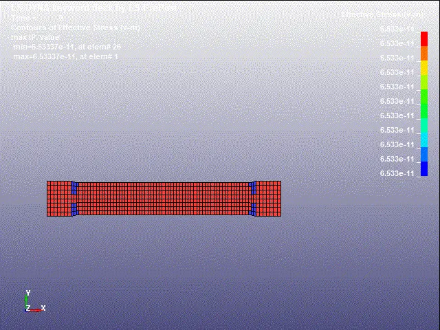
From this we need to select a random element in the middle to plot the true stress and true strain values from which engineering stress and strain can be calculated

• Validation for Case 2: In the *MAT_HYPERELASTIC_RUBBER_ by keeping N=0 we can input the mooney-rivlin constants obatined during case 2

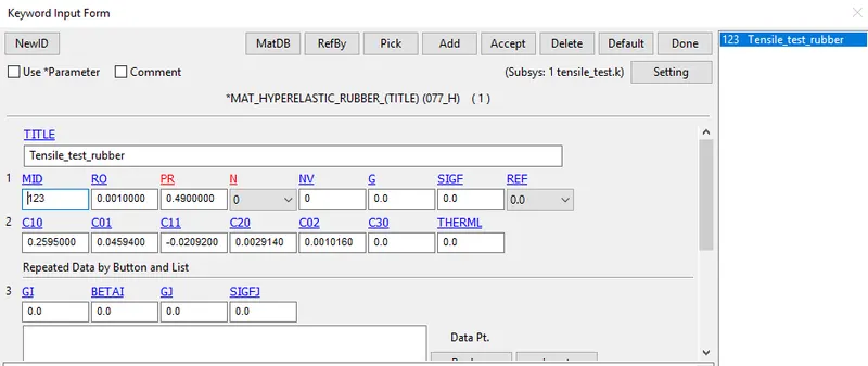
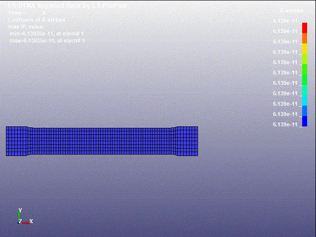
From this we need to select a random element in the middle to plot the true stress and true strain values from which engineering stress and strain can be calculated

• Validation for Case 3: In the *MAT_HYPERELASTIC_RUBBER_ by keeping N=0 we can input the mooney-rivlin constants obatined during case 3

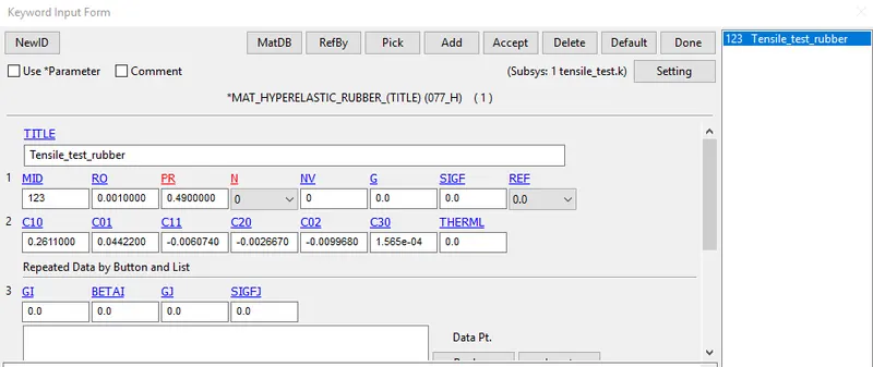
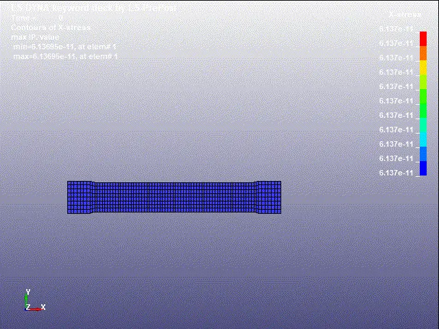
From this we need to select a random element in the middle to plot the true stress and true strain values from which engineering stress and strain can be calculated.

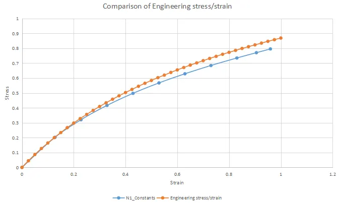
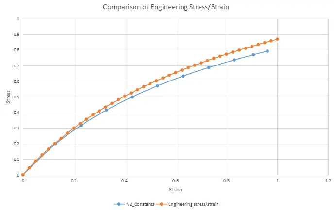
From the obtained true stress and strain the Engineering stress and strain values are caluculated for all the three cases and the calculated value is plotted which is then compared with the original data from the material curve.

Graph:

Case 1:

Case 2:

Case 3:

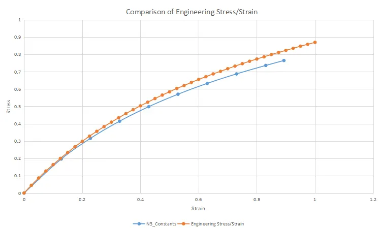
• Here we can see that there is an exact corelation between the experimental data and the raw data in all the three cases
• but due to some non linearities there is some deviation, which is acceptable.

Conclusion:

From the given raw data image of Engineering Stress/Strain, material curve data is extracted and material model for MAT_77 _HYPERELASTIC_RUBBER_ card is created and results are plotted then corelated with the raw data plot to be validated.