Week - 10 Hyperelastic Material Models

Hyper-elastic Material Models

Objective

• Given raw material data, calculate the Mooney Rivlin and Ogden material constants
• Validate the both models using a tensile test simulation with a 100% strain value

Background

Hyper-elastic materials, also known as elastomers, are characterized by exhibiting large elastic deformations when subjected to relatively low external forces. This behavior is possible due to the entanglement and reorientation of the long polymer chains that constitute these types of materials

Some of the most common hyper-elastic materials include: Natural rubber, synthetic rubber, silicone rubber, polyurethane and thermoplastics. Yet, unlike linear elastic materials such as metals, hyper-elastic materials do not follow Hooke's Law and therefore it's very complex to model their stress/strain relationships.

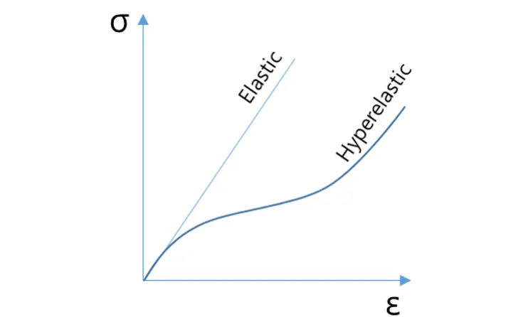
Two of the most popular material models to represent this complex behavior are the Mooney Rivlin and Ogden models. Both of them describe the strain energy density of the materials as a function of their principal stretches, yet, they differ in the sense that they do a different fit.

The Mooney Rivlin model uses a polynomial series in the form of:

Where W is the strain energy density, C1 and C2 are fitted material constants, and I1 and I2 are the strain invariants derived from the principal stretches

In contrast, the Ogden Model describes the strain energy density as a power-law function of the principal stretches:

Where represents the principal stretch ratios, and and are fitted constants

Procedure

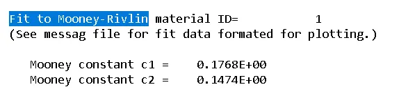
In order to calculate the Mooney Rivlin and Ogden material constants Ls-Dyna provides an in-built model for hyper-elastic materials known as MAT077

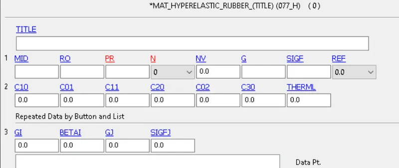
By defining a curve with the engineering stress-strain data obtained from a uniaxial tensile test Ls-Dyna can calculate all the material constants with different models by varying the N value between 1,2 and 3.

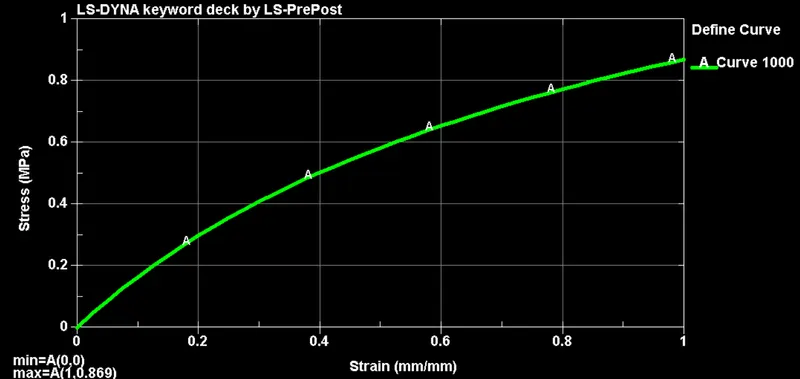
The resultant material card with rubber material properties is shown in the next figure:

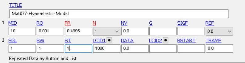
From there, we simply have to run the model and check for the fitted constants at the

d3hsp file

In order to verify the accuracy of the fitted model, we can also used the extension (stretch) and true stress obtained from the fit and plot against the original stress-strain plot.

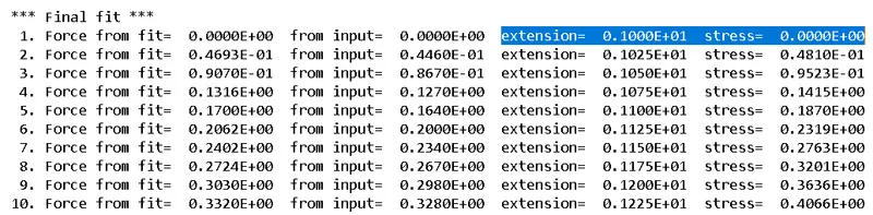
The stretch can be converted into engineering strain by using the following equation:

Meanwhile, the true stress can be converted into engineering stress by using:

The comparison between the original raw data and the Mooney Rivlin model can be observed in the following figure:

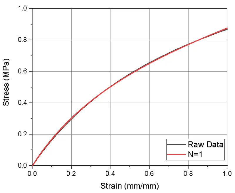
As observed, the fitted model is very accurate since the maximum strain is relatively low for a hyper-elastic material. The same procedure will be carried out using N = 2 and N = 3 , which will yield the fitted constants to use an Ogden material model with 2 and 3 terms, respectively. The summary of the results can be observed in the following table/figure:

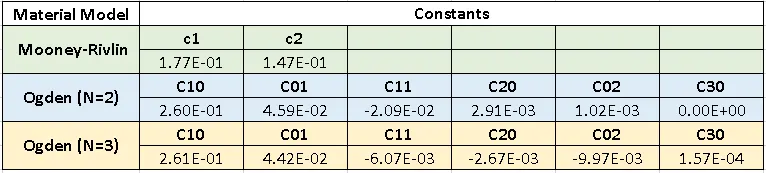
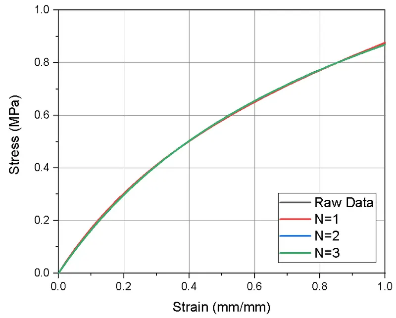
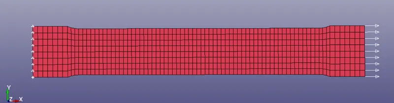
All the models yielded a very accurate fit, so, the next step is to validate the model using a uniaxial test simulation with all the material models. To do so, the following model (with a 5mm thickness) is used:

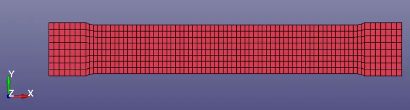
The boundary conditions used for this model include:

• A prescribed motion of 145mm in the right hand side nodes (which has to be applied by using a define curve keyword)

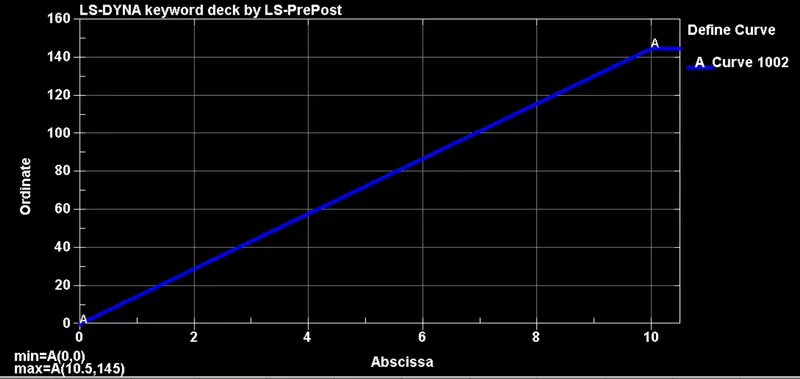
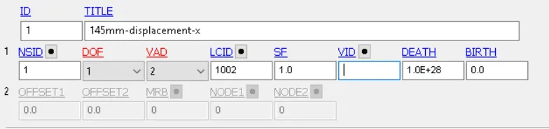
• Fixed translations in the X and Z axis, as well as fixed rotations in all axes for the edge nodes

• Fixed Y translation for the middle nodes of the tensile test specimen

Since this simulation can be considered as quasi-static, a implicit simulation scheme is more accurate. We can specify this solution scheme in Ls-Dyna by activating the following set of keywords:

• Control Implicit General ---> Activates Implicit solution scheme
• Control Implicit Auto --> Enables auto time step adjustment during the simulation
• Control Implicit Solution --> Enables the non-linear solver
• Control Implicit Solver --> Enable the liner solver

We also have to input the material model constants according to the model we want to use.

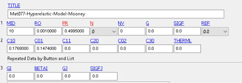
For the Mooney Rivlin model we have to input C10 and C01

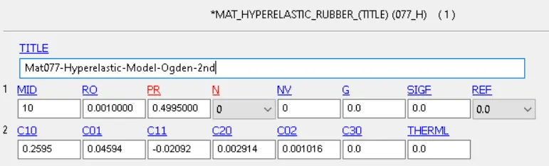
For the 2nd order Ogden model we use all constants as shown in the following figure

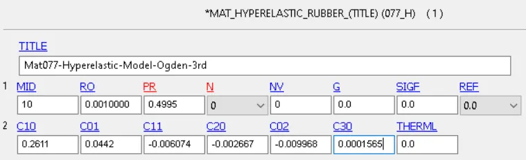
Similarly, we also use all constants for the 3rd order Ogden model

Simulation Results

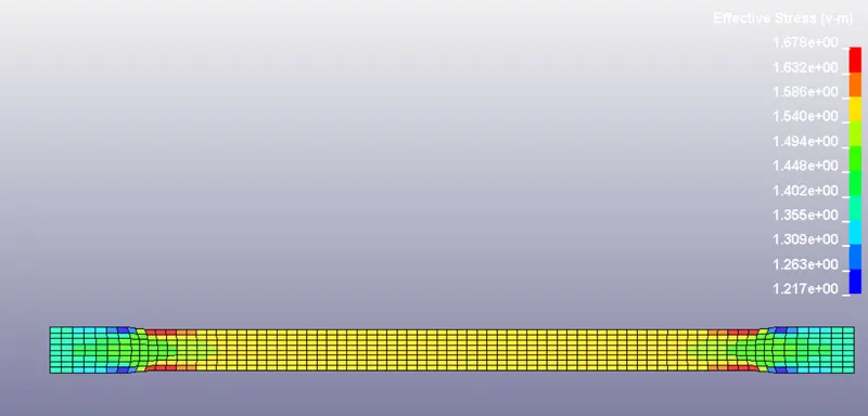
All the simulations yield the same stress/strain distribution in which the higher stresses are located near the fillets, which act as a stress concentration point. This can be observed in both the following image/video

The correlation between all the material models and the raw data can be observed in the following figure

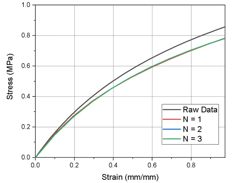
As observed, all of the models behave similarly since the strain values are relatively low for a hyper-elastic material. Particularly, 3rd order Ogden model has shown to be effective up to 700% strain.

The difference between our model and the experimental data can be attributed to several factors such as:

• Geometry of the test specimen (thickness, size, features)
• Material properties (Poisson's ratio and density)
• Mesh quality and refinement

Conclusions

• Both Mooney Rivlin and Ogden material models are very effective at representing highly complex hyper-elastic materials

• The correlation of the model may be improved by varying the geometry of the tensile test, the material properties and even the mesh of the component