Week 1 - Plot function using basic Simulink blocks

AIM :

To plot function `y(x)=(x−1)⋅(x−3)^2⋅(x−9)^2` using basic Simulink blocks and run suspension system comparison.

OBJECTIVES :

• To create fundamental Simulink blocks using a given function.
• To run Simulink example for Suspension System Comparison.

GOVERNING EQUATION :

`y(x)=(x−1)⋅(x−3)^2⋅(x−9)^2`

SIMULINK :

It is a MATLAB-based graphical programming environment that is used for modeling, simulating and analyzing multidomain dynamical systems. It provides a graphical editor, customizable block libraries, and solvers for modeling and simulating dynamic systems. It is integrated with MATLAB, enabling you to incorporate MATLAB algorithms into models and export simulation results to MATLAB for further analysis.

SIMULINK BLOCK :

EXPLANATION :

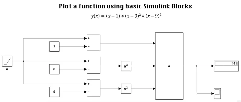
1. From the given function, we first sorted out all the required Simulink blocks. The required blocks are ramp, constants, subtracts, squares, product, scope and display.
2. Ramp block acts as a multiplier for various values.
3. This ramp is well connected with all the subtracting blocks with their respective constants & making substracting blocks as (x-1), (x-3) & (x-9).
4. Two blocks are squared using square blocks.
5. Further, all three blocks are well connected to the product block having three inputs and giving one output.
6. The output or result from the product block is shown in the display block. Here the output is realised in terms of the 'y' variable.
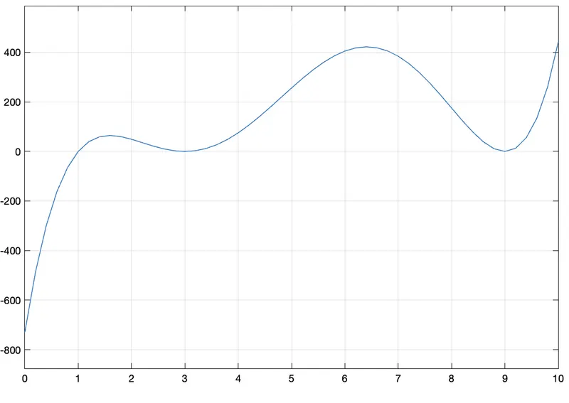
7. Finally, the scope block is used to show the output in terms of values.

SCOPE :

SUSPENSION SYSTEM COMPARISION :

THEORY :

This example shows a testbed containing three sets of springs and dampers excited by the same oscillating velocity source. The first uses the Shock Absorber block and includes linear stiffness and damping. Optional friction and hard stops are not used. The second shock absorber uses a Nonlinear Translational Spring and a Nonlinear Translational Damper specified by symmetric polynomials. The third uses a Variable Translational Spring and Variable Translational Damper. The spring constant is varied during the simulation using open-loop control and the damping coefficient adjusts to ensure critical damping is achieved. Closed-loop control can be added to simulate an adaptive suspension system.

MODEL :-

OUTPUT :

I. Simulation Results from Simscape Logging :-

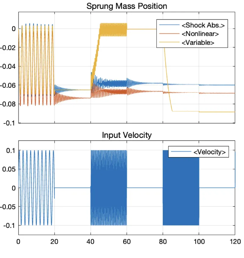
The plot below shows the position of the sprung masses in three different suspension models that are subjected to the same test.

II. Power Spectral Density :-

Q & A :

A. What is the objective of the simulation? What are the similarities and differences between the three systems understudy?

Objectives :

• To run a real-world suspension system with the help of Simulink software.
• To compare and analyse the suspension system with the help of plot (consisting of shock absorber spring, non-linear spring & variable spring which are well connected at the end to give us the output).

Similarities :

• The velocity source is the same for all three systems.
• It also has tire stiffness, sprung mass & unsprung mass in common.

Differences :

• The spring and damping parameters are different for all the systems.
• The first uses the Shock Absorber block and includes linear stiffness and damping. Optional friction and hard stops are not used.
• The second shock absorber uses a Nonlinear Translational Spring and a Nonlinear Translational Damper specified by symmetric polynomials.
• The third uses a Variable Translational Spring and Variable Translational Damper.

B. What are your observations from the results?

• From the graph, we have observed that the input oscillating frequency starting at 3rad/sec the time from 0-20 sec is the same for all three systems in terms of the sprung mass position.
• After increasing the frequency to 15rad/sec, we can see the changes from 40-60 sec, the sprung mass position shows very minimal vibration for variable spring as compared to that of the shock absorber & non-linear spring.
• After increasing further the frequency to 75rad/sec, we observed changes from 80-100 sec, the variable spring reaches its minimum vibration position which is around -0.09, whereas the other two show more vibration and the minimum position of the shock absorber spring and non-linear spring is at -0.06 & -0.07 respectively.

C. How the oscillating velocity source is created?

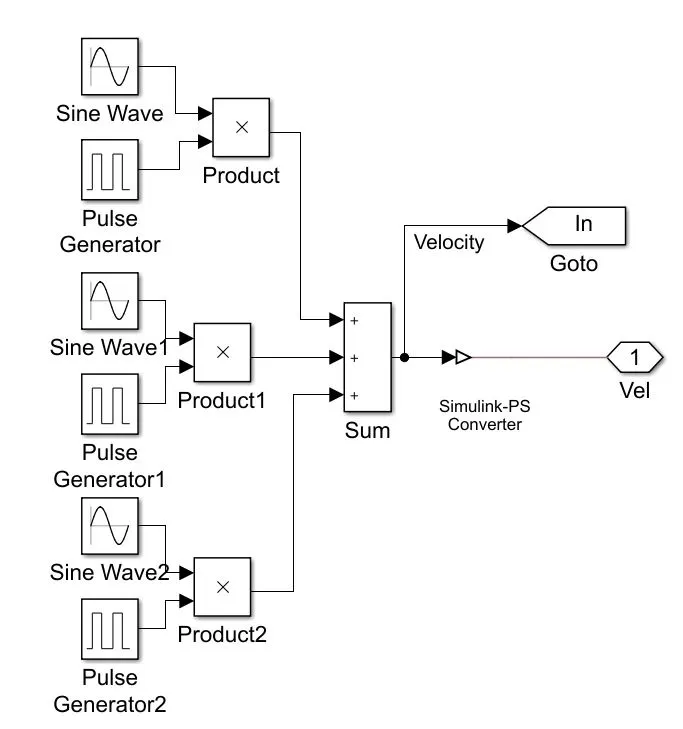
The oscillating velocity source is created with three sine waves with different frequencies along with three pulse generators. They are 3 rad/sec, 15 rad/sec, 75 rad/sec respectively. The time period for each oscillation is given as 20 seconds. The blocks diagram is shown in the above figure. Next, a sine wave and pulse generator are connected to give us the product in the form of a new velocity of x. The same process is repeated for the next 2 & 3 blocks. Later they are sum (with three inputs) which gives us the final result in the form of a velocity signal.

CONCLUSION :

• From the function, we have created the Simulink blocks and found its output value which is 441 and plotted it in the form of a graph.
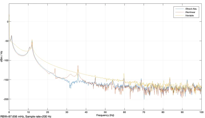
• For Suspension System Comparison, we have run the model to get its sprung mass position, input velocity and power spectral density to get its results & plot them in the form of graphs. The vibration of the suspension system for all three springs is then observed.

REFERENCES :

• How to plot and get the output for an equation using Simulink?
• Suspension System Comparison